
Finding a Quadratic Function with a Minimum Point
Loading the math board and drawing, please wait…
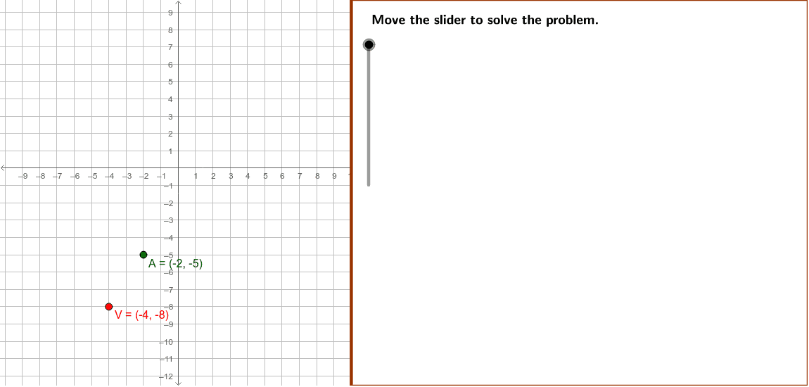
This example demonstrates how to determine the equation of a quadratic function with a specified minimum point and passing through a given point. Key math concepts include quadratic functions, vertex coordinates, function graphing, and coordinate geometry. GeoGebra commands like If, Polygon, and TableText are utilized in the construction. Suitable for high school students learning about quadratic functions and their graphs.
GeoGebra Commands & Parameters
If(x(B) ≟ x(A), B + (1, 0), B) → VPolygon((edge, y(Corner[1])), Corner[2], Corner[3], (edge, y(Corner[4]))) → Mask, mask1, mask2, mask4, mask3If(abs(b) ≟ 1, If[b ≟ 1, "", "-"], LaTeX[b]) → b1If(abs(c) ≟ 1, If[c ≟ 1, "", "-"], LaTeX[c]) → c1TableText({{"\textit{f}(\textit{x})=\textit{a}(\textit{x} " + (LaTeX[Element[plus, sgn((-x(V))) + 2]]) + "" + (LaTeX[(-x(V))]) + " )^2" + (LaTeX[Element[plus, sgn(y(V)) + 2]]) + "" + (LaTeX[y(V)]), " \text{Equation from step 1.}"}, {" \textit{f}(\textit{x})= \frac{" + (LaTeX[y(A) - y(V)]) + "}{" + ((LaTeX[x(A)^(2)] * "}(\textit{x} ")) + (LaTeX[Element[plus, sgn((-x(V))) + 2]]) + "" + (LaTeX[(-x(V))]) + " )^2 " + (LaTeX[Element[plus, sgn(y(V)) + 2]]) + "" + (LaTeX[y(V)]), " "}}, "l") → Conclusions3TableText({{"\textit{f}(\textit{x})= \textit{a}(\textit{x}-\textit{h})^2+\textit{k}", " \text{Vertex form}"}, {" \textit{f}(\textit{x})=\textit{a}[\textit{x}-(" + (LaTeX[x(V)]) + ")]^2+(" + (LaTeX[y(V)]) + ") ", "\text{Substitute " + (LaTeX[V]) + " for } \textit{h}\text{ and }\textit{k}."}, {" \textit{f}(\textit{x})=\textit{a} (\textit{x}" + (LaTeX[Element[plus, sgn((-x(V))) + 2]]) + "" + (LaTeX[(-x(V))]) + ")^2" + (LaTeX[Element[plus, sgn(y(V)) + 2]]) + "" + (LaTeX[y(V)]), "\text{Simplify.}"}}, "l") → Conclusions1TableText({{"\textit{f}(\textit{x})=\textit{a}(\textit{x}" + (LaTeX[Element[plus, sgn((-x(V))) + 2]]) + " " + (LaTeX[(-x(V))]) + ")^2 " + (LaTeX[Element[plus, sgn(y(V)) + 2]]) + " " + (LaTeX[y(V)]), "\text{Equation from step 1.} "}, {LaTeX[y(A)] + "=\textit{a}[(" + (LaTeX[x(A)]) + ")" + (LaTeX[Element[plus, sgn((-x(V))) + 2]]) + " " + (LaTeX[(-x(V))]) + "]^2" + (LaTeX[Element[plus, sgn(y(V)) + 2]]) + " " + (LaTeX[y(V)]), "\text{Substitute }" + (LaTeX[A]) + "\text{ for } \textit{x} \text{ and }\textit{f}(\textit{x}). "}, {LaTeX[y(A)] + "=a[" + (LaTeX[x(A)]) + "]^2" + (LaTeX[Element[plus, sgn(y(V)) + 2]]) + "" + (LaTeX[y(V)]), "\text{Simplify.}"}, {LaTeX[y(A)] + "=" + (LaTeX[x(A)^(2)]) + "\textit{a}" + (LaTeX[Element[plus, sgn(y(V)) + 2]]) + "" + (LaTeX[y(V)])}, {LaTeX[y(A) - y(V)] + "=" + (LaTeX[x(A)^(2)]) + "\textit{a}", " "}, {" \frac{" + (LaTeX[y(A) - y(V)]) + "}{" + (LaTeX[x(A)^(2)]) + "}=\textit{a} ", " "}}, "l") → Conclusions2
AI Drawing Prompt Reference
Draw the graph of a quadratic function with a specified vertex point and passing through another given point. First, mark the vertex and the given point, then plot the function graph. Next, use the polygon tool to connect the vertex and key points on the graph, forming an auxiliary shape. Finally, label the vertex form equation of the function and its derivation process next to the graph, including the coefficients obtained from the vertex coordinates and the given point coordinates.
The prompt above was compiled from the original drawing commands and is for reference only.