Filling a Cone: Dynamic Water Level and Volume Simulation

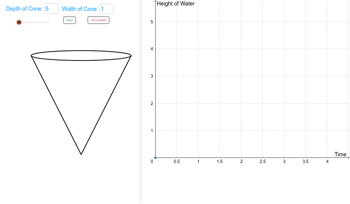
① This GeoGebra example dynamically simulates filling a conical container with water, visually demonstrating how the water level rises over time and how the surface area and volume change. ② Core mathematical concepts include the cone volume formula, proportional relationships, function graphs (water height vs. fill amount), and interactive elements like sliders and input fields. ③ Construction highlights: commands such as Tangent, Function, and Polygon are used to build the cone's side and base; Textfield and input boxes (inputBox1, inputBox2, inputBox3) control fill parameters; sliders (depth, width, radius) adjust cone dimensions; buttons (button1, button2) trigger the filling animation; Polygon and point objects (P1, watertopfill) render the water surface. ④ Suitable for middle and high school geometry and algebra lessons, especially for understanding cone volume formulas, function modeling, and the power of dynamic visualization in mathematics education.