Field Goal Angle and Parabolic Trajectory Exploration

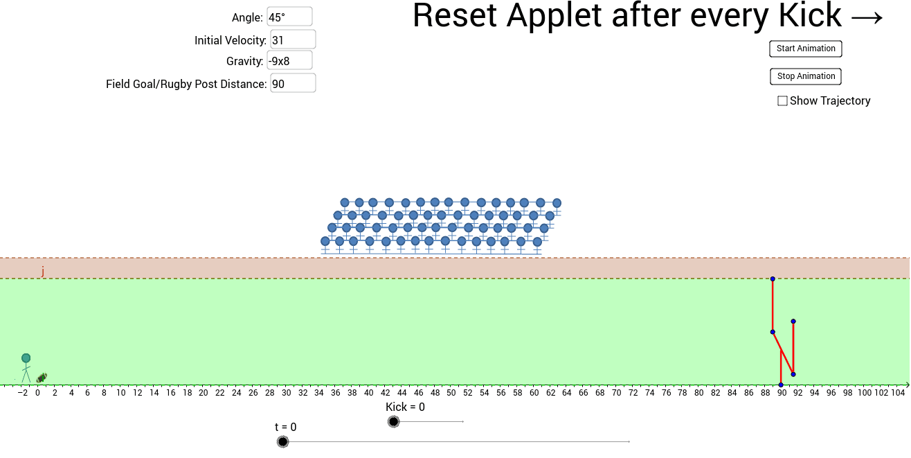
This example uses a football field goal scenario to demonstrate how to determine the optimal kicking angle for accurate shots. Key mathematical concepts include: (1) quadratic functions for modeling parabolic trajectories; (2) trigonometric functions for calculating incidence and azimuth angles; (3) geometric transformations using Rotate and Dilate commands to visualize the ball's flight path; (4) construction elements like orthocenter and parallelogram for geometric relationships. Construction details: The GeoGebra construction uses input boxes (inputBox1-4) for interactive parameter adjustment, sliders (α, rad1, rad2) for dynamic angle control, text fields for displaying real-time calculations, and transformation commands (Rotate, Dilate) for animating the trajectory. Suitable for high school mathematics classes teaching quadratic function applications, trigonometric practice, and optimization problems, as well as introductory mathematical modeling learners understanding parametric approaches.