
Fascinating Properties of Conic Sections: From 3D Cone to 2D Cuts
Loading the math board and drawing, please wait…
In collections
Conic Sections
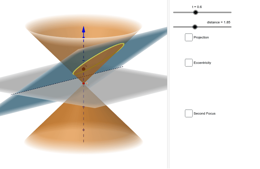
This applet demonstrates remarkable properties of conic sections based on Alexander Givental's paper 'Kepler's Laws and conic sections'. It visualizes how a plane cutting an infinite cone yields ellipses, hyperbolas, or parabolas as the plane's orientation changes, connecting to Kepler's laws of planetary motion. Core mathematical concepts include the unified definition of conics, foci and directrices, eccentricity, symmetry, and the intersection of planes with surfaces. The construction employs GeoGebra commands such as InfiniteCone, Plane, IntersectPath, LineBisector, OrthogonalLine, Locus, Surface, and OrthogonalPlane to create the cone, cutting plane, intersection curves, and auxiliary elements like foci and directrices. This is ideal for high school to university-level geometry instruction, particularly for analytic geometry, solid geometry, and interdisciplinary astronomy-physics learning, offering a three-dimensional insight into the intrinsic relationships among conic sections.
GeoGebra Commands & Parameters
InfiniteCone((0, 0, 0), Vector[(0, 0, 0), (0, 0, 1)], 0.7853981633974483) → coneLine(C, D) → bLine(B, b) → aPlane(a, b) → cIntersectPath(g, c) → iIntersectPath(g, cone) → qIntersect(i, q) → E, FLineBisector(E, F, g) → fIntersect(f, yAxis) → F_2IntersectPath(c, cone) → dPoint(d) → MLocus(G, M) → loc1Point(loc1) → JOrthogonalLine(J, b, space) → f_1Intersect(f_1, b) → HSegment(J, H) → deSegment(J, F_1) → nuPoint(loc1) → PIntersectPath(g, cone) → rLine(F_1, (0, 0, 1)) → jIntersectIntersect(q, r) → A, , ,Intersect(f, j) → OSurface((t * cos(u)), (t * sin(u)), (t^(2) - ((2 * t) * h) + ((4 * p) * k) + h^(2)) / ((4 * p)), t, -15, 15, u, 0, 6.28319) → l_1Segment(M, F) → mSegment(M, F) → nSegment(E, F) → sOrthogonalLine(F_2, xAxis, g) → a_2Point(xAxis) → H_1Line(H_1, F_2) → b_1OrthogonalLine(F_2, b_1, g) → c_1Intersect(c_1, s) → QSegment(F_2, P) → d_1Segment(F_1, P) → d_2Intersect(zAxis, c) → NOrthogonalLine(J, xy) → e_1Line(M, G) → gmLine(Q, F_2) → g_1OrthogonalPlane(O, j) → oIntersectPath(o, cone) → h_1Intersect(c_1, c) → IIntersect(c_1, c) → K
AI Drawing Prompt Reference
Visualize an infinite 3D cone and a plane intersecting it to produce ellipses, hyperbolas, or parabolas depending on the plane's orientation. Show how changing the plane angle alters the intersection curves, highlighting key elements like foci, directrices, and eccentricity. Include symmetry axes, perpendicular bisectors, and auxiliary planes, along with the locus of intersection points between the curves and the cone surface, linking conic sections to Kepler's laws of planetary motion.
The prompt above was compiled from the original drawing commands and is for reference only.