
Exponential and Logarithmic Functions: Graphs and Relationships
Loading the math board and drawing, please wait…
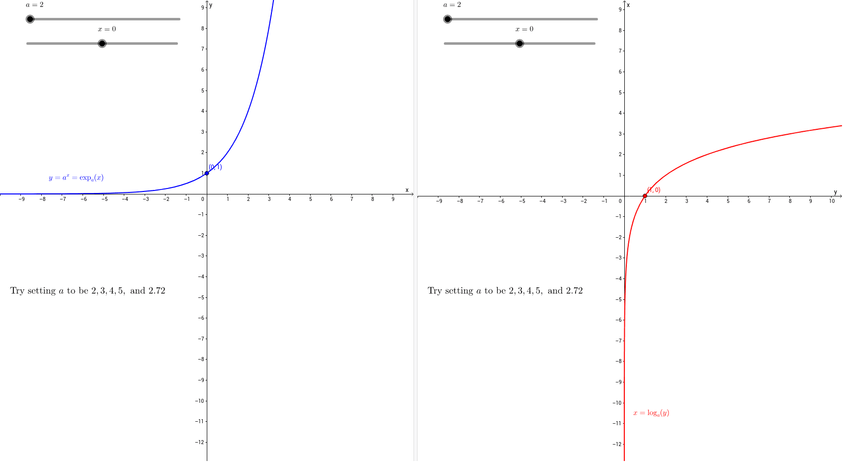
This GeoGebra example dynamically illustrates the graphs of exponential and logarithmic functions, which are inverses of each other, and their reflection symmetry about the line y=x. Core mathematical concepts include exponential functions, logarithmic functions, inverse functions, reflection transformations, and the effect of base parameters on graph shape. Construction highlights: using adjustable parameters a and b, defining functions f (exponential) and g (logarithmic), creating points A and B with their corresponding relationships, and using text objects text1, text2, and text1_1 to label key points or equations. Suitable for high school or pre-university students learning function properties, inverse functions, and graph transformations, as well as for exploring dynamic changes with varying bases.
GeoGebra Commands & Parameters
Numeric a(2.0)Numeric b(0.0)f(x) = a^(x)g(x) = log(a, x)(b, a^(b))(a^(b), b)
AI Drawing Prompt Reference
Draw a coordinate plane with an exponential curve and its inverse logarithmic curve, symmetric about the line y=x. The exponential function has a variable base a, and the logarithmic function uses the same base. Place a point on the exponential curve at x-coordinate b, with y-coordinate a^b. Place the corresponding point on the logarithmic curve at x-coordinate a^b, with y-coordinate b. Label both points with their coordinates and show the function equations. Use sliders to adjust parameters a and b, and observe how the curves and points change dynamically.
The prompt above was compiled from the original drawing commands and is for reference only.