
Exploring Pi
Loading the math board and drawing, please wait…
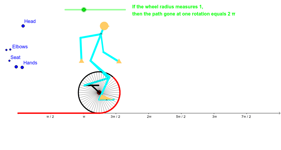
This example dynamically demonstrates the ratio of a circle's circumference to its diameter, visually showcasing the constancy and calculation of Pi. It involves core mathematical concepts like circle, rotation, dilation, Pythagorean theorem, combinatorics, and intersection calculations. Construction highlights the use of commands such as Circle, Point, Rotate, CircleArc, Intersect, Segment, Line, Vector, Translate, Polygon, and Sequence in GeoGebra. Suitable for high school mathematics education to understand basic circle properties and the practical application of Pi.
GeoGebra Commands & Parameters
Circle(A, 1) → cPoint(c) → BRotate(B, (-a), A) → B'CircleArc(A, B, B') → dIntersect(xAxis, yAxis) → DSegment(D, B) → bPoint(yAxis) → CPoint(b) → ECircle(C, E) → ePoint(c) → FLine(F, A) → fPoint(f) → GCircle(A, 0.5) → gSegment(G, A) → hRotate(f, (-a), A) → f'Intersect(g, f', 1) → HIntersect(g, f', 2) → ISegment(H, A) → iSegment(I, A) → jLine(H, xAxis) → kLine(I, xAxis) → lPoint(k) → KPoint(k) → MPoint(l) → NPoint(l) → OSegment(O, N) → mSegment(M, K) → nCircle(M, 1.2) → qVector((0, 0), (a, 0)) → uTranslate(L, u) → L'Circle(L', 1.2) → rIntersect(q, r, 2) → PSegment(M, P) → pSegment(L', P) → sCircle(O, 1.2) → tIntersect(r, t, 1) → QSegment(O, Q) → a_1Segment(L', Q) → b_1Translate(R, u) → R'Circle(R', 0.2) → d_1Segment(R', L') → c_1Point(c_1) → STranslate(T, u) → T'Translate(U, u) → U'Segment(S, T') → e_1Segment(S, U') → f_1Translate(W, u) → W'Translate(V, u) → V'Segment(T', W') → g_1Segment(U', V') → h_1Rotate(S, a / 4, S) → S'Rotate(S', sin(a), S) → S''Polygon(S, W', T') → poly1, t', s_1, w'Rotate(S, sin((2 * a)), S'') → S'_1Rotate(S, sin(a), S'') → S'_2Rotate(W', sin(a), S'') → W''_1Rotate(T', sin(a), S'') → T''_1Polygon(S'_2, W''_1, T''_1) → poly1', t''_1, s'_2, w''_1Polygon(V', U', S) → poly2, s_2, v', u'Rotate(V', (-sin(a)), S'') → V''Rotate(U', (-sin(a)), S'') → U''Rotate(S, (-sin(a)), S'') → S'_3Polygon(V'', U'', S'_3) → poly2', s'_3, v'', u''Segment(W''_1, T''_1) → i_1Segment(T''_1, S) → j_1Segment(S, U'') → k_1Segment(V'', U'') → l_1Segment(U'', V'') → m_1Point(p) → ZPolygon(K, M, Z) → poly3, z_1, k_2, m_2Rotate(S, (0.5 * sin((2 * a))), S'') → S'_4Rotate(W', (0.5 * sin((2 * a))), S'') → W''Rotate(T', (0.5 * sin((2 * a))), S'') → T''Polygon(S'_4, W'', T'') → poly1'_1, t'', s'_4, w''Point(a_1) → A_1Polygon(O, N, A_1) → poly4, a_2, o, n_1Point(c) → B_1Sequence(Rotate[B_1, (π / 24 * n), A], n, 1, 49) → list1Sequence(Segment[Element[list1, n], A], n, 1, 49) → list2Sequence(Rotate[Element[list2, n], (-a), A], n, 1, 49) → list3Circle((0, 1), 1) → p_1Point(xAxis) → D_1Segment(C_1, D_1) → q_1Point(d_1) → E_1
AI Drawing Prompt Reference
Draw a circle and mark its center and diameter. Mark two points on the diameter, rotate one point, and draw the arc formed. Find the intersection point of the coordinate axes and connect it to one of the points on the circle. Mark another point on the circle, connect it to the center, and draw the perpendicular line. Draw a circle with the center as the origin and half the radius of the original circle. Find the intersection points of this circle with the perpendicular line. Connect the intersection points to the center. Draw a line segment between two points on the perpendicular line. Draw a larger circle with one of the intersection points as the center. Draw a vector from the original center and translate the original circle along this vector to draw a new circle. Find the intersection points of the two circles and connect each intersection point to its corresponding center. Repeat this process for the other intersection point. Draw a larger circle with one of the intersection points as the center. Find the intersection points of this new circle with the translated circle and connect each intersection point to its corresponding center. Repeat this process for the other intersection point.
The prompt above was compiled from the original drawing commands and is for reference only.