Exploring Hyperbola Properties: Foci, Asymptotes, and Geometric Construction

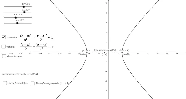
① This GeoGebra example dynamically demonstrates the core properties of a hyperbola, including its foci, transverse and conjugate axes, asymptotes, and the geometric relationships of points on the curve. ② The key mathematical concepts covered are the standard equation of a hyperbola, foci and eccentricity, asymptote equations, the defining property that the difference of distances from any point on the hyperbola to the two foci is constant, and auxiliary constructions (triangles, parallelograms) built from orthogonal lines and intersections to aid visualization. ③ Construction highlights: Based on the construction summary, the example uses GeoGebra commands such as OrthogonalLine, Intersect, Segment, and Line, creating numerous points (A₂, B₁, C, D, E, F, G, J, K, N, O), lines (d, f, g, i, e, c, w, f₁, g₁, h₁, i₁), and text objects (text1–text8). Parameters a, b, h, k control the hyperbola equation, allowing dynamic exploration of how changing these values affects the curve and its associated geometric elements. ④ Target audience: High school analytic geometry (conic sections) or introductory college geometry courses; ideal for classroom demonstrations, student self-exploration of hyperbola properties, or as a template for teachers creating interactive instructional materials.