
Example QF.2.3
Loading the math board and drawing, please wait…
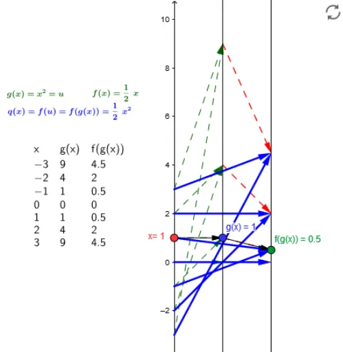
This example demonstrates the graph and properties of quadratic equations. Key mathematical concepts include quadratic equations, function graphs, and linear regression. Using GeoGebra commands such as Point, Vector, and Textfield, the example dynamically shows the graph and related properties of quadratic equations. Suitable for middle and high school mathematics education.
GeoGebra Commands & Parameters
Point(yAxis) → AVector(A, B) → uVector(B, C) → vTextfield(g) → inputBox1Textfield(f) → inputBoxfSequence(-3, 3, dx) → NZip(Vector[(2, g(z)), (4, f(g(z)))], z, N) → fgx_*Zip(Vector[(0, z), (2, g(z))], z, N) → g_*Zip((z, g(z)), z, N) → Pg_*Zip((z, f(g(z))), z, N) → Pfg_*Zip(Vector[(0, z), (4, f(g(z)))], z, N) → qx_*TableText(Transpose[{Append["x", N], Append["g(x)", g(N)], Append["f(g(x))", f(g(N))]}]) → Table
AI Drawing Prompt Reference
Draw a graph of a quadratic function and show its relationship with linear regression. First, plot the curve of the quadratic function on a coordinate system. Then, add an input box for linear regression parameters. Next, dynamically generate points for the quadratic function at different x values and label them. Finally, compare these points with the fitted line of linear regression to help understand the properties of the quadratic function and the application of linear regression.
The prompt above was compiled from the original drawing commands and is for reference only.