
Euler's Method Tool
Loading the math board and drawing, please wait…
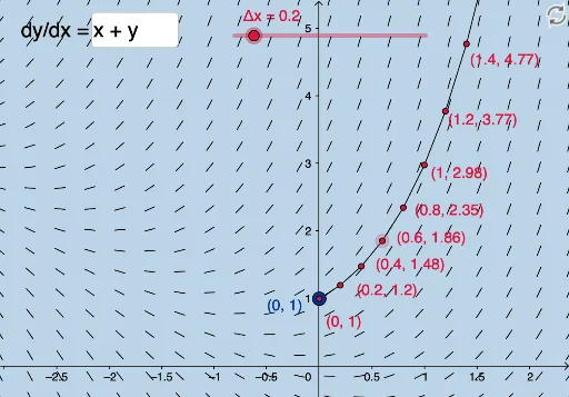
This example demonstrates the numerical approximation process of solving differential equations using Euler's method. Key math concepts include differential equations, numerical methods, and function iteration. Construction highlights involve using SlopeField for direction fields, PolyLine for approximate solution curves, and Textfield for displaying parameters and results, with objects like A1, dx, Δx, f. Suitable for high school students and teachers to understand numerical methods for differential equations and visualization.
GeoGebra Commands & Parameters
SlopeField(f, 20) → slopefield1PolyLine({B, C, D, E, F, G, H, I, J, K, L, M, N, O, P, Q, R, S, T, U, V, W, Z, A_1, B_1, C_1, D_1, E_1, F_1, G_1, H_1, I_1, J_1, K_1, L_1, M_1, N_1, O_1, P_1, Q_1, R_1, S_1, T_1, U_1, V_1, W_1, Z_1, A_2, B_2, C_2}) → aTextfield(f) → InputBox1
AI Drawing Prompt Reference
Create a graph illustrating Euler's method for numerically solving differential equations. Start by drawing a slope field on the coordinate plane, with short line segments indicating the slope direction at various points. Then, from an initial point, construct a polyline connecting successive points obtained by Euler's method with a fixed step size, forming an approximate solution curve that traverses the slope field. Finally, include an input box near the graph to display or edit the differential equation, allowing dynamic updates to the curve. The layout should clearly show the relationship between the numerical approximation and the direction field.
The prompt above was compiled from the original drawing commands and is for reference only.