
Estimating Pi using Pick's Theorem
Loading the math board and drawing, please wait…
In collections
Pi Approximations
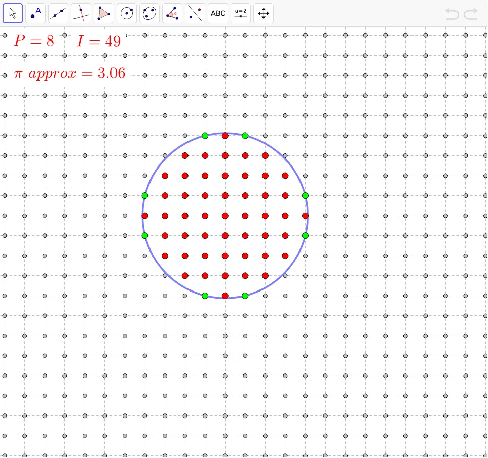
This example dynamically demonstrates the application of Pick's Theorem in geometric figures to estimate Pi. It involves core mathematical concepts such as Pick's Theorem, polygon area, and counting interior and boundary dots. The construction uses GeoGebra commands like Join, Circle, Sequence, and Sum. Suitable for high school and above, it helps learners understand Pick's Theorem and its use in approximation calculations.
GeoGebra Commands & Parameters
Join(Sequence[Sequence[(i, j), j, -20, 20], i, -40, 40]) → DotsCircle(A, B) → cSequence(Distance[A, Element[Dots, k]], k, 1, Length[Dots]) → DistanceFromDotsSum(Sequence[If[Element[DistanceFromDots, k] ≟ Radius[c], 1, 0], k, 1, Length[DistanceFromDots]]) → PerimeterDotsSum(Sequence[If[Element[DistanceFromDots, k] < Radius[c], 1, 0], k, 1, Length[DistanceFromDots]]) → InteriorDotsSequence(Sequence[If[sqrt((i - xA)^(2) + (j - yA)^(2)) < Radius[c], (i, j)], j, -20, 20], i, -40, 40) → ShowInteriorDotsSequence(Sequence[If[sqrt((i - xA)^(2) + (j - yA)^(2)) ≟ Radius[c], (i, j)], j, -20, 20], i, -40, 40) → ShowBoundaryDots