Dynamic Visualization of Polynomial Roots and Geometric Construction

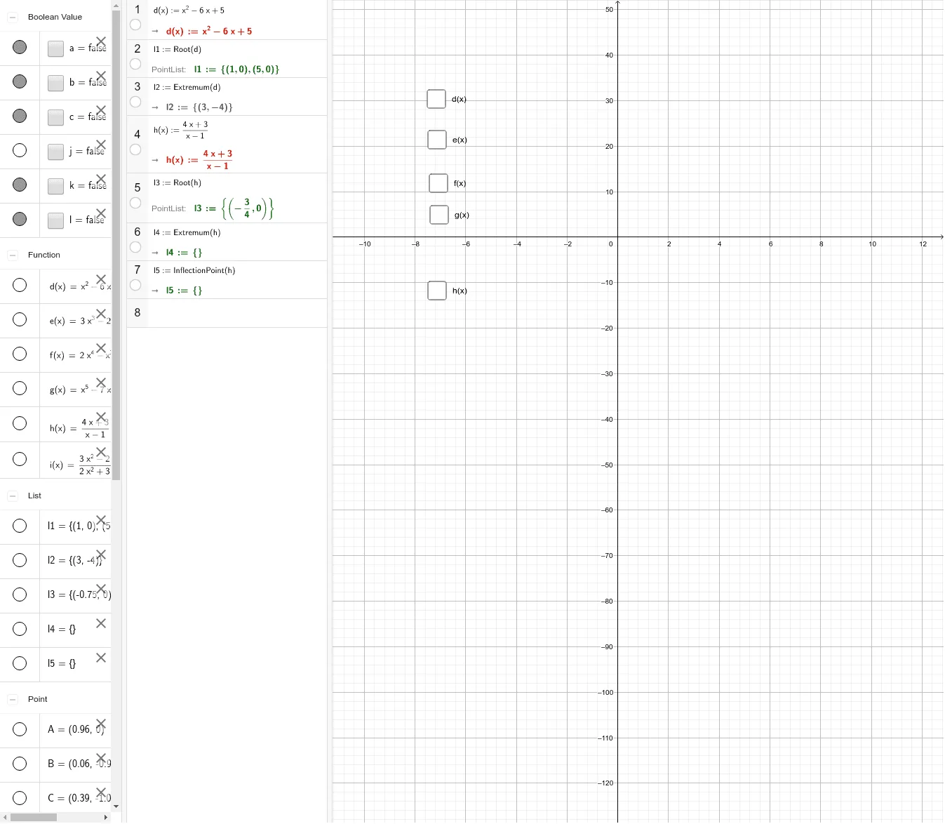
This GeoGebra example demonstrates the dynamic solving of polynomial roots while integrating diverse mathematical elements such as rhombus, vectors, normal distribution, and differential equations, creating a comprehensive interactive exploration environment. The core mathematical concepts include polynomial roots (Root), extrema (Extremum), and turning points (TurningPoint), along with their geometric correspondences on the function graph. The construction utilizes commands like Root, Extremum, and TurningPoint to precisely mark key points, and employs objects such as l1, d, l2, e to build auxiliary shapes, while linking numerous point objects (A through S) and function objects (f, g, h) to enable real-time updates of root positions as parameters change. This example is suitable for high school to undergraduate mathematics instruction, particularly in courses covering functions and equations, analytic geometry, and mathematical modeling, helping students intuitively grasp the distribution patterns of polynomial roots and their connection to graphical features.