
Domain and Range of Square Root Functions
Loading the math board and drawing, please wait…
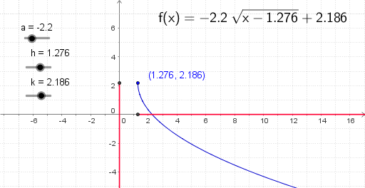
This example dynamically demonstrates the domain and range of square root functions using GeoGebra. It covers core concepts like function graphs, domain (x≥0), range (y≥0), and function transformations. Key GeoGebra commands and objects used include Point, OrthogonalLine, Intersect, Ray, If, and parameters h, k, a, C, f, T1, B, D, E, F, d, e, G, A, I, g, q for parametric manipulation. Suitable for high school mathematics education to understand function properties and graph transformations.
GeoGebra Commands & Parameters
Point(yAxis) → BPoint(yAxis) → DPoint(xAxis) → EPoint(xAxis) → FOrthogonalLine(C, yAxis) → dOrthogonalLine(C, xAxis) → eIntersect(e, xAxis) → GIntersect(d, yAxis) → APoint(xAxis) → IRay(G, I) → gIf(a > 0, Ray[A, B], If[a ≟ 0, Ray[A, A], Ray[A, D]]) → q
AI Drawing Prompt Reference
Draw the graph of a square root function to show its domain and range. Start by creating points B and D on the y-axis, and points E and F on the x-axis. Then create perpendicular lines d and e through point C, and find their intersections with the x-axis and y-axis, G and A. Draw a ray g from G to I. Finally, based on the value of parameter a, draw different rays q: if a is greater than 0, draw a ray from A to B; if a equals 0, draw a ray from A to A; if a is less than 0, draw a ray from A to D.
The prompt above was compiled from the original drawing commands and is for reference only.