
Domain and Range of Cube Root Functions
Loading the math board and drawing, please wait…
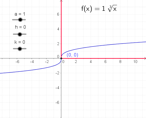
This example illustrates the domain and range of cube root functions. It involves key mathematical concepts such as functions, root operations, and parametric curves. Using GeoGebra commands like Point, OrthogonalLine, and Intersect, the function graph and its properties can be dynamically demonstrated. Suitable for high school mathematics education and learning.
GeoGebra Commands & Parameters
Point(yAxis) → BPoint(yAxis) → DPoint(xAxis) → EPoint(xAxis) → FOrthogonalLine(C, yAxis) → dOrthogonalLine(C, xAxis) → eIntersect(e, xAxis) → GIntersect(d, yAxis) → APoint(xAxis) → IRay(G, I) → gIf(a > 0, Ray[A, B], If[a ≟ 0, Ray[A, A], Ray[A, D]]) → q
AI Drawing Prompt Reference
Draw the graph of a cube root function to illustrate its domain and range. Mark points on the x-axis and y-axis, then draw perpendicular and horizontal lines from these points, marking the intersections. Extend a ray from the intersection along the x-axis to the right, determining its starting point based on the function's parameter. Finally, choose different ray drawing methods based on the parameter's sign to dynamically demonstrate the function's properties.
The prompt above was compiled from the original drawing commands and is for reference only.