
Discovering Average Rate of Change of a Function
Loading the math board and drawing, please wait…
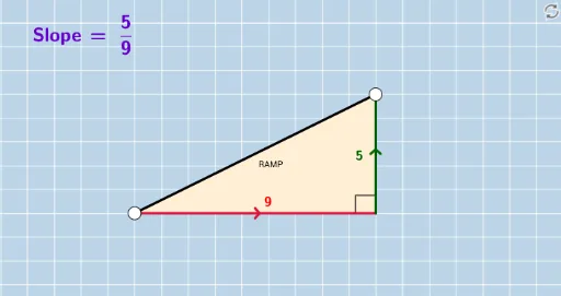
This example demonstrates how to dynamically visualize the average rate of change of a function using GeoGebra. Core math concepts involved include function graphs, slope, difference calculation, and rate of change. Construction highlights extract commands/objects like GCD (Greatest Common Divisor), If (Conditional), OrthogonalLine (Perpendicular Line), Intersect (Intersection), Line (Line Segment), Polygon (Polygon), Distance (Distance), Segment (Segment), Angle (Angle), and Slope (Slope) from the 'Construction Summary'. Suitable for high school mathematics students to understand the concept of function rate of change and slope, as well as introductory calculus knowledge.
GeoGebra Commands & Parameters
GCD(deltaY, deltaX) → GCDmGCD(numerYint, deltaX) → GCDyIf(sgn(deltaY / deltaX) ≥ 0, "", "-") → textSignNIf(sgn(numerYint / deltaX) > 0, "+", "-") → textSignIf(deltaXR ≟ 1, textSignN + deltaYR, textSignN + "\, \frac{" + deltaYR + "}{" + deltaXR + "}") → textslopeNIf(denomYintR ≟ 1, textSign + numerYintR, textSign + "\frac{" + numerYintR + "}{" + denomYintR + "}") → textYintIf(denomYintR ≟ 1, If[numerYintR ≟ 1, textSign, textSign + numerYintR], textSign + "\frac{" + numerYintR + "}{" + denomYintR + "}") → textMIDOrthogonalLine(B, xAxis) → a_2OrthogonalLine(A, yAxis) → cIntersect(a_2, c) → CLine(A, B) → dPolygon(A, B, C) → poly1, c_1, a_1, b_1Distance(B, C) → distanceBCDistance(A, C) → distanceACIntersect(a_2, c) → DSegment(A, D) → eSegment(C, B) → fGCD(deltaY_1, deltaX_1) → GCDm_1If(sgn(deltaY_1 / deltaX_1) ≥ 0, "", "-") → textSignN_1If(deltaXR_1 ≟ 1, textSignN_1 + deltaYR_1, textSignN_1 + "\, \frac{" + deltaYR_1 + "}{" + deltaXR_1 + "}") → textslopeN_1Line(A_1, B_1) → d_1Angle(B, D, A) → αSegment(A, B) → gGCD(deltaY_2, deltaX_2) → GCDm_2If(sgn(deltaY_2 / deltaX_2) ≥ 0, "", "-") → textSignN_2If(deltaXR_2 ≟ 1, textSignN_2 + deltaYR_2, textSignN_2 + "\, \frac{" + deltaYR_2 + "}{" + deltaXR_2 + "}") → textslopeN_2Line(A_2, B_2) → d_2Segment(A_2, B_2) → g_1GCD(deltaY_3, deltaX_3) → GCDm_3If(sgn(deltaY_3 / deltaX_3) ≥ 0, "", "-") → textSignN_3If(deltaXR_3 ≟ 1, textSignN_3 + deltaYR_3, textSignN_3 + "\, \frac{" + deltaYR_3 + "}{" + deltaXR_3 + "}") → textslopeN_3Line(A_3, B_3) → d_3Segment(A_3, B_3) → g_2Slope(g) → h
AI Drawing Prompt Reference
Draw a function graph and select two points A and B on it. Draw a line d through A and B. Construct a triangle with points A, B, and C, and calculate the lengths of AB and BC. Construct a perpendicular line a_2 from A to the x-axis, and another perpendicular line c from B to the y-axis, which intersect at point C. Calculate the slope and label it on the graph. Find the midpoint D of A and B, draw segments AD and BC, and calculate angle α. Draw the segment g between A and B, and calculate its slope.
The prompt above was compiled from the original drawing commands and is for reference only.