Direction Fields and Solution Curves: Geometric Visualization of Differential Eq

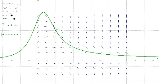
① This example demonstrates how to visualize the solution curves of a first-order differential equation using direction fields (slope fields), allowing users to adjust parameters and observe how the solution changes with initial conditions. ② Core mathematical concepts include differential equations, direction fields, slope fields, numerical integration (e.g., Euler or Runge-Kutta methods), and the geometric interpretation of solution curves. ③ Construction highlights: The GeoGebra command SlopeField generates the direction field; Textfield and input boxes (inputBox1 to inputBox5) provide interactive control over the differential equation expression, domain ranges, and initial point; the Locus command traces the solution curve; numericalIntegral1 performs numerical solving; a slider (delta) controls step size; A denotes the initial point, resulting in a dynamic, explorable interface. ④ Suitable for advanced high school or early university calculus and differential equations courses, this example helps students grasp the existence and uniqueness of solutions, the relationship between direction fields and solution curves, and supports mathematical experimentation or inquiry-based learning.