
Dirac Delta and Limiting Heaviside Functions
Loading the math board and drawing, please wait…
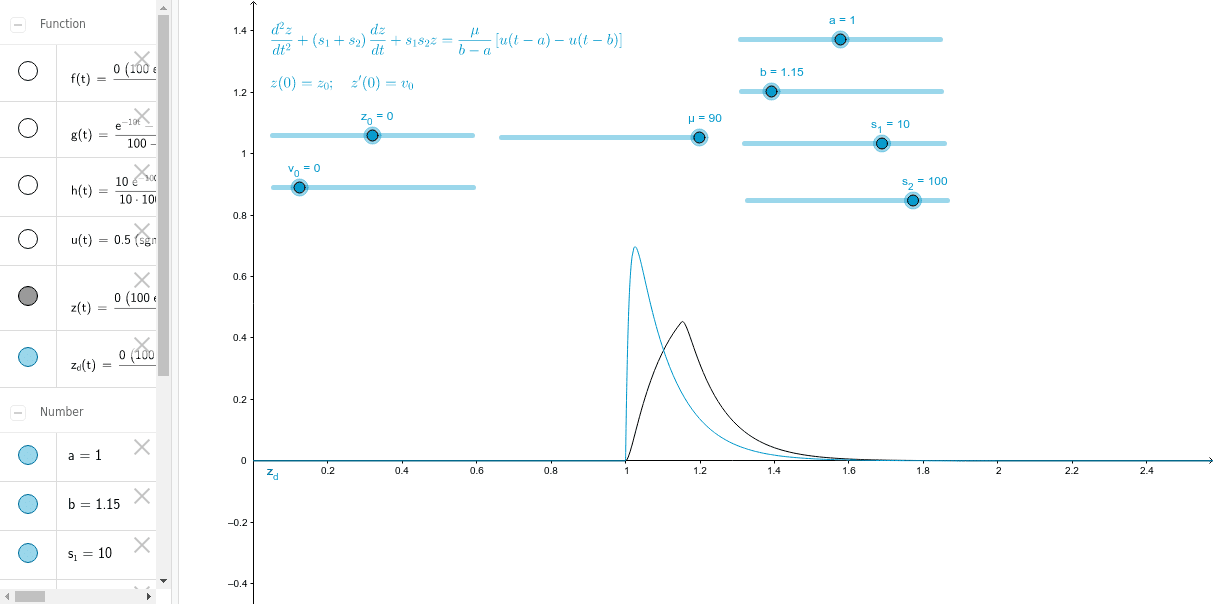
This GeoGebra example visualizes the Dirac delta function and its relationship to the Heaviside step function through a limiting process. It demonstrates how a sequence of smooth or piecewise functions, parameterized by a slider, converges to the idealized delta distribution, while the step function emerges as its integral. Core mathematical concepts include generalized functions, distribution theory, the derivative of the step function, and the concept of limits in function spaces. The construction uses the Function command to define multiple objects (f, h, g, z) and auxiliary parameters (a, b, μ, z_0, v_0, s_1, s_2) to build approximating curves, with text4 labeling key formulas. This is ideal for university-level calculus, mathematical physics, or signal processing courses, as well as for advanced high school students exploring the intuitive meaning of delta functions and limits.
GeoGebra Commands & Parameters
Function(((z_0 * ((s_2 * ℯ^((-10 * t))) - (s_1 * ℯ^((-100 * t))))) + (v_0 * (ℯ^(((-s_1) * t)) - ℯ^(((-s_2) * t))))) / (s_2 - s_1), 0, 3) → fFunction(((s_1 * ℯ^(((-s_2) * t))) - (s_2 * ℯ^(((-s_1) * t)))) / (((s_1 * s_2) * (s_2 - s_1))) + 1 / ((s_1 * s_2)), 0, 3) → hFunction((ℯ^(((-s_1) * t)) - ℯ^(((-s_2) * t))) / (s_2 - s_1), 1, 3) → gFunction(f(t) + (μ * ((u(t - a) * h(t - a)) - (u(t - b) * h(t - b))) / (b - a)), 0, 3) → zFunction(f(t) + ((μ * u(t - a)) * g(t - a)), 0, 3) → z_d
AI Drawing Prompt Reference
Create a graph illustrating the limiting relationship between the Dirac delta and Heaviside step functions. Over the interval 0 to 3, use sliders to control two decay parameters, and plot three curves: one for displacement response, one for step response, and one for impulse response. Then overlay a modified curve combining a rectangular pulse with step functions, and a variant with a single-sided step. Label key formulas with text, showing how a sequence of smooth functions approaches the ideal delta distribution, whose integral yields the step function.
The prompt above was compiled from the original drawing commands and is for reference only.