
Differential Equations: Mapping Diagram, Slope Field, Solution
Loading the math board and drawing, please wait…
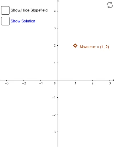
This example demonstrates the graphical representation of mapping diagrams, slope fields, and solutions for differential equations. Key math concepts include differential equations, vector fields, slope fields, and numerical solution methods. It utilizes GeoGebra commands like If, SolveODE, Sequence, Vector, Segment, and Textfield. Suitable for high school and above students to understand the geometric meaning and numerical solutions of differential equations.
GeoGebra Commands & Parameters
If(var ≟ 2, P, f') → f_qSolveODE(f_q, (a, y0)) → hSequence(0, N) → NLVector(B, C) → uVector(C, DEvecpt) → DEvecSegment(E, F) → gTextfield(f') → InputBox2If(var ≟ 2, SlopeField[f_q, N + 5, 3], SlopeField[f', N + 5, 3]) → slopefield1If(var ≟ 2, f_q, f') → P1Textfield(P) → inputBox1_2Textfield(y0) → InputBox1Segment(x', B) → jVector(x', y') → vTextfield(a) → inputBox2Vector(x', Solmd) → w
AI Drawing Prompt Reference
Create a visual representation showing vector fields, slope fields, and solutions to differential equations, starting with the derivative function and key points, then solving the differential equation numerically for solution curves, generating vector fields and slope fields, and finally integrating all elements in a coordinate system with labeled parameters and derivative functions.
The prompt above was compiled from the original drawing commands and is for reference only.