
Derivative Practice: Sections 2.3-2.5
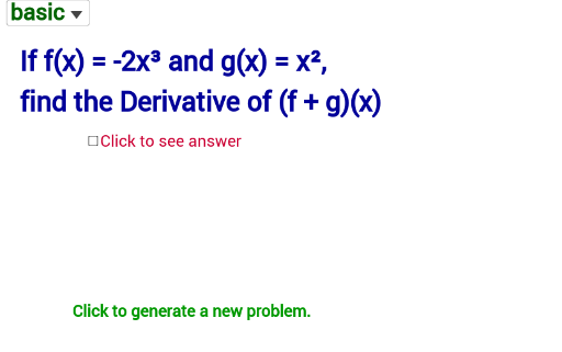
Loading the math board and drawing, please wait…
This example demonstrates content from Sections 2.3-2.5 of the derivative practice, involving key concepts such as derivatives and indefinite integrals. Using GeoGebra commands like RandomElement, Random, and Join, dynamic function graphs and their properties are showcased. Suitable for high school math education and learning.
GeoGebra Commands & Parameters
RandomElement({-4, -3, -2, -1, 1, 2, 3, 4}) → a1RandomElement({-4, -3, -2, -1, 1, 2, 3, 4}) → a2Random(1, 5) → oppickJoin({bflist, First[cflist, SelectedIndex[ftype] - 1]}) → flistRandomElement(flist) → cRandomElement(flist) → dRandomElement({-3, -2, -1, 2, 3}) → c1Element({c(x) + d(x), c(x) - d(x), (c(x) * d(x)), c(x) / d(x), c(d(x))}, oppick) → e1Simplify(e1) → fElement(oplist, oppick) → oppickedIf(B1 > 0, N1) → A4Simplify(Derivative[e1]) → gLaTeX(g) → text3
AI Drawing Prompt Reference
Draw a function f(x) and its derivative g(x). f(x) is constructed by combining two random polynomial functions c(x) and d(x) using addition, subtraction, multiplication, or division. g(x) is the derivative of f(x). Show the graphs of f(x) and g(x), and their properties such as monotonicity and extreme points.
The prompt above was compiled from the original drawing commands and is for reference only.