
Derivative Machine
Loading the math board and drawing, please wait…
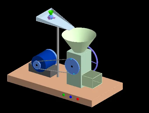
This example treats 'Derivative' as an operator that transforms one function into another. By analogy with an input-output machine, we explore the concept of derivatives. Using GeoGebra commands such as Line, Circle, Point, etc., we construct the graph of a function and the geometric meaning of its derivative. Suitable for high school mathematics education, particularly for learning calculus and function graphs.
GeoGebra Commands & Parameters
Line(O_1, P_1) → f_2Circle(I_2, 1.7, f_2) → d_3Point(d_3) → P_2Polygon(A, B, C, D) → poly1, a_5, b, c, dPrism(poly1, 0.8519331046338638) → e, E, edgeAE, edgeBF, edgeCG, edgeDH, edgeEF, edgeFG, edgeGH, edgeEH, F, G, H, faceABFE, faceBCGF, faceCDHG, faceADHE, faceEFGHPolygon(I, J, K, L) → poly2, i, j, k, lPrism(poly2, 5) → f, M, edgeIM, edgeJN, edgeKO, edgeLP, edgeMN, edgeNO, edgeOP, edgeMP, N, O, P, faceIJNM, faceJKON, faceKLPO, faceILPM, faceMNOPCone(R, Q, 2) → g, h, mPoint(k) → SPoint(k) → VPolygon(S, T, U, V) → poly3, s, t, u, vPrism(poly3, 1.2) → n, W, edge1, edge2, edge3, edge4, edge5, edge6, edge7, edge8, Z, A_1, B_1, face1, face2, face3, face4, face5Prism(face5, -1.2646911609860731) → o, C_1, edge9, edge10, edge11, edge12, edge13, edge15, edge16, edge14, D_1, E_1, F_1, face6, face8, face9, face7, face10Cylinder(G_1, H_1, 1) → p, q, r, wCylinder(I_1, J_1, 1) → a_1, a_2, a_3, a_4Cylinder(K_1, L_1, 0.5) → b_1, c_1, d_1, e_1Cylinder(K_1, L_1, 0.45) → f_1, g_1, h_1, i_1Cylinder(G_1, K_1, 0.15) → j_1, j_2, j_3, j_4Midpoint(O_1, P_1) → R_1Midpoint(K_1, L_1) → T_1Line(K_1, L_1) → n_1Circle(n_1, U_1) → t_1Circle(f_2, S_1) → c_2Tangent(c_2, t_1) → r_1, s_1, g_2, h_2Intersect(-6.4380165289256395x² + 61.98347107438032x y - 128.132231404959y² - 10.04132231404962x + 41.838842975206745y = 3.388946280991749, x² + y² = 0.8100000000000006) → , , ,Intersect(s_1, c_2) → V_1, W_1Intersect(s_1, t_1) → Z_1, A_2Intersect(r_1, t_1) → B_2, C_2Intersect(r_1, c_2) → D_2, E_2Segment(A_2, W_1) → i_2Segment(C_2, E_2) → l_2Circle(G_2, 0.15) → d_2Polygon((x(G_2) - 2, y(G_2) - 1.5, 8), (x(G_2) + 2, y(G_2) - 0.5, 7.5), (x(G_2) + 2, y(G_2) + 0.5, 7.5), (x(G_2) - 2, y(G_2) + 1.5, 8)) → poly4, m_2, n_2, p_2, q_2Polygon((x(G_2) - 2, y(G_2) - 1.5, 8), (x(G_2) - 2, y(G_2) - 1.5, 8.5), (x(G_2) - 2, y(G_2) + 1.5, 8.5), (x(G_2) - 2, y(G_2) + 1.5, 8)) → poly5, r_2, s_2, t_2, b_2Polygon((x(G_2) - 2, y(G_2) - 1.5, 8), (x(G_2) + 2, y(G_2) - 0.5, 7.5), (x(G_2) - 2, y(G_2) - 1.5, 8.5)) → poly6, f_3, g_3, h_3Polygon((x(G_2) - 2, y(G_2) + 1.5, 8), (x(G_2) + 2, y(G_2) + 0.5, 7.5), (x(G_2) - 2, y(G_2) + 1.5, 8.5)) → poly7, i_3, l_3, m_3Cylinder(d_2, 7.6) → u_1, u_2, u_3Cylinder(M_1, O_1, 0.1) → o_1, e_2, c_3, v_1Rotate(P_2, a / 2, f_2) → J_2Rotate(J_2, π / 3, f_2) → K_2Rotate(K_2, π / 3, f_2) → L_2Rotate(L_2, π / 3, f_2) → M_2Rotate(M_2, π / 3, f_2) → N_2Rotate(N_2, π / 3, f_2) → O_2Cylinder(I_2, J_2, 0.05) → w_2, q_3, r_3, v_2Cylinder(I_2, O_2, 0.05) → w_1, w_4, w_5, w_6Cylinder(I_2, M_2, 0.05) → w_3, w_7, w_8, w_9Cylinder(I_2, L_2, 0.05) → o_3, o_3, o_4, o_5Cylinder(I_2, N_2, 0.05) → g_4, g_5, g_6, g_7Cylinder(I_2, K_2, 0.05) → b_3, b_4, b_5, b_6Cylinder(O_1, P_1, 1) → l_1, l_4, l_5, l_6Cylinder(O_1, P_1, 0.9) → k_1, k_2, k_3, k_4Rotate(A_2, a, n_1) → Q_2Rotate(C_2, a, n_1) → T_2Rotate(W_1, a / 2, f_2) → S_2Rotate(E_2, a / 2, f_2) → R_2Dilate(A_2, p_1, W_1) → V_2Dilate(C_2, (-p_1) - 0.5, E_2) → W_2Cylinder(I_2, O_1, 0.15) → q_1, q_4, q_5, q_6Line(A_3, xAxis) → n_3Point(n_3) → B_3OrthogonalLine(B_3, n_3) → p_3OrthogonalLine(A_3, n_3) → s_3Point(s_3) → C_3OrthogonalLine(C_3, s_3) → t_3Intersect(p_3, t_3) → D_3Polygon(A_3, B_3, D_3, C_3) → poly8, a_6, b_7, d_4, c_4Prism(poly8, 1.8) → o_2, E_3, edge17, edge18, edge19, edge20, edge21, edge22, edge23, edge24, F_3, G_3, H_3, face11, face12, face13, face14, face15Midpoint(n_2) → J_3Line(R, (0, 0, 0)) → f_4Line(J_3, f_4) → h_4Point(h_4) → L_3Dilate(L_3, v_3 - 1, J_3) → M_3Midpoint(B_1, C_1) → N_3Line(N_3, edgeEH) → i_4Point(i_4) → O_3Line(I_3, Q_3) → e_3Dilate(Q_3, v_3, I_3) → K_3Textfield(p_4) → InputBox2Dilate(O_3, (v_3 - 3) / 2, N_3) → P_3PointIn(faceKLPO) → T_3OrthogonalLine(T_3, faceKLPO) → s_4Line(K_3, edgeNO) → f_5Line(K_3, edgeLP) → h_5Sphere(K_3, 0.3) → d_5Point(h_5) → V_3Cone(V_3, K_3, 0.3) → e_5, k_5, i_5Point(f_5) → W_3Cylinder(K_3, W_3, 0.1) → j_5, p_5, r_5, m_5Sphere(M_3, 0.3) → s_5Line(M_3, h_5) → f_6Point(f_6) → Z_3Cone(Z_3, M_3, 0.3) → u_5, c_6, v_5Line(M_3, f_5) → h_6Point(h_6) → A_4Cylinder(M_3, A_4, 0.1) → d_6, e_6, k_6, i_6Line(K_3, edgeOP) → j_6Point(j_6) → B_4Line(M_3, edgeOP) → m_6Point(m_6) → C_4Circle(B_4, 0.2, j_6) → p_6Circle(C_4, 0.2, m_6) → r_6Line(P_3, edgeLP) → n_6Point(n_6) → D_4Midpoint(D_4, P_3) → E_4Cylinder(D_4, P_3, 0.3) → o_6, s_6, c_7, u_6Point(n_6) → F_4Cone(F_4, E_4, 0.3) → v_6, d_7, a_7Line(E_4, i_4) → f_7Point(f_7) → G_4Cylinder(E_4, G_4, 0.1) → e_7, h_7, k_7, i_7Line(E_4, edgeOP) → j_7Point(j_7) → H_4Circle(H_4, 0.2, j_7) → p_7Midpoint(edge6) → I_4Line(I_4, edge7) → l_7Line(P_3, edge11) → m_7Intersect(m_7, l_7) → J_4Vector(P_3, J_4) → u_7Translate(o_6, u_7) → n_7Translate(a_7, u_7) → o_7Translate(p_7, u_7) → q_7Translate(i_7, u_7) → r_7Derivative(p_4) → dr
AI Drawing Prompt Reference
Draw the graph of a function and its derivative. Start by plotting the function curve, then draw a circle with the curve as its boundary. Next, create a cylinder with the circle as its boundary, ensuring the cylinder's axis is tangent to the curve. Extend small cones upward from the cylinder, forming a stepped appearance. Finally, add several small cylinders to the side of the cylinder to enrich the structure.
The prompt above was compiled from the original drawing commands and is for reference only.