
Degrees of Freedom Distribution in Linkages
Loading the math board and drawing, please wait…
In collections
Linkages
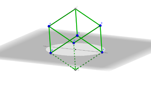
This example demonstrates the distribution of degrees of freedom in linkage mechanisms and their geometric relationships. Core math concepts include geometric constructions, coordinate geometry, and probability & statistics. Construction highlights involve commands like Segment, Point, Circle, and IntersectConic to build the geometric model. Suitable for high school students and math enthusiasts studying kinematics and geometric modeling.
GeoGebra Commands & Parameters
Segment((-1, 0, 0), (1, 0, 0)) → sAPoint(sA) → ACircle(OO, abs(A), zAxis) → dePoint(de) → EPoint(de) → UIntersectConic(Sphere[U, 1], Sphere[E, 1]) → cUEIntersectConic(Sphere[U, 1], Sphere[A, 1]) → cUAIntersectConic(Sphere[E, 1], Sphere[A, 1]) → cEAPoint(cUA) → BPoint(cEA) → DPoint(cUE) → FIntersectConic(Sphere[B, 1], Sphere[D, 1]) → cBDIntersectConic(Sphere[B, 1], Sphere[F, 1]) → cBF
AI Drawing Prompt Reference
In 3D coordinate space, draw a horizontal segment of length 2 with two fixed endpoints as base points. From one endpoint, construct a circle in a vertical direction using the distance from the origin as its radius, then pick two distinct points on that circle. Model linkage geometry using spheres: for each chosen point, take a sphere of radius 1 and compute pairwise intersections between these spheres to form several space intersection curves. From the intersections, identify the corresponding key points and continue intersecting with other radius‑1 spheres to obtain the remaining points. Present the resulting point configuration and the geometric relationships implied by the multiple sphere–sphere intersections to visualize the distribution of degrees of freedom in a linkage mechanism.
The prompt above was compiled from the original drawing commands and is for reference only.