
Damped Harmonic Motion - Displacement vs Time Plot
Loading the math board and drawing, please wait…
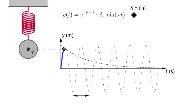
This example demonstrates the displacement vs time plot of a damped harmonic oscillator. It involves exponential and trigonometric functions, and key mathematical concepts like differential equations. GeoGebra commands and objects used include Function, Point, OrthogonalLine, Intersect, Circle, Vector, Segment, Polygon, and Spring. Suitable for high school physics and mathematics education to understand vibration damping phenomena.
GeoGebra Commands & Parameters
Function(ℯ^(-δ * x) * amplitude * sin(omega * x), tmin, t) → gPoint(xAxis) → EOrthogonalLine(E, xAxis) → aOrthogonalLine(D, yAxis) → cIntersect(a, c) → FFunction(amplitude * sin(omega * x), tmin, tmax) → fCircle(F, radius) → d_1Vector((0, 0), (tmax + offset, 0)) → uVector((0, 0), (0, amplitude + offset)) → vVector(((3 * π / 2) / omega, -amplitude - offset / 2), ((7 * π / 2) / omega, -amplitude - offset / 2)) → zVector(((7 * π / 2) / omega, -amplitude - offset / 2), ((3 * π / 2) / omega, -amplitude - offset / 2)) → eFunction(amplitude * ℯ^(-δ * x), tmin, tmax) → hSegment(F, D) → dPoint(a) → AOrthogonalLine(A, a) → bCircle(A, 1.25) → kIntersect(k, b) → B, CIntersect(d_1, a) → G, HPoint(a) → IOrthogonalLine(B, b) → iOrthogonalLine(I, a) → jOrthogonalLine(C, b) → lIntersect(l, j) → JIntersect(j, i) → KPolygon(C, J, K, B) → Vieleck1, c_1, j_1, k_1, b_1Spring(H, A, n, r, strut) → m, L, f_1, M, N, p, q, o, s, a_1, e_1