
Cylinder Volume Exploration Module 8B (Pri Hastuti Suryaningrum, SMPN 57)
Loading the math board and drawing, please wait…
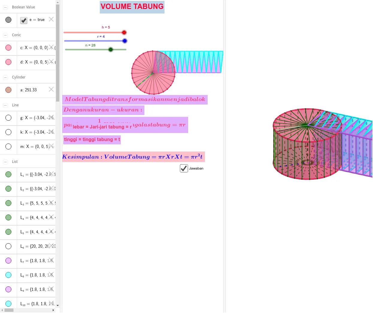
① This GeoGebra example dynamically demonstrates the volume formula of a cylinder, allowing users to adjust the radius r and height h via sliders to observe real-time changes in volume. ② Core mathematical concepts include the cylinder volume formula V=πr²h, solid geometry, parameter-dependent volume variation, and an intuitive connection to integration as a sum of infinitesimal layers. ③ Construction highlights: from the summary, the example uses the Cylinder command to create the solid, along with Point, Segment, Line, Intersect, Polygon, Sequence, and OrthogonalLine to build auxiliary geometry, while sliders (r, h) control dimensions; multiple labeled objects (L_1 to L_8) display computed values. ④ Suitable for middle or early high school students, this resource supports teaching of solid geometry and volume formulas, and can be used for classroom demonstrations or self-guided exploration.
GeoGebra Commands & Parameters
Cylinder(A, B, r) → a, c, d, bPoint(d) → CSegment(B, C) → fLine(C, zAxis) → gSegment(A, B) → iIntersect(g, c, 1) → DSegment(A, D) → jPolygon(A, B, C, D) → q1, a_1, b_1, c_1, d_1Sequence(Rotate[C, ((i * 360) * ° / n), B], i, 0, n) → L_1Sequence(Rotate[D, ((i * 360) * ° / n), A], i, 0, n) → L_2Sequence(Segment[Rotate[C, ((i * 360) * ° / n), B], Rotate[D, ((i * 360) * ° / n), A]], i, 0, n) → L_3Sequence(Segment[Rotate[B, ((i * 360) * ° / n), B], Rotate[C, ((i * 360) * ° / n), B]], i, 0, n) → L_4Sequence(Segment[Rotate[A, ((i * 360) * ° / n), B], Rotate[D, ((i * 360) * ° / n), B]], i, 0, n) → L_5Line(C, D) → kSequence(Rotate[q1, ((i * 360) * ° / n), j], i, 0, n) → L_6Point(L_1) → GSegment(C, G) → lOrthogonalLine(B, l, space) → mIntersect(m, l) → HSegment(B, H) → pSegment(C, G) → dxSegment(B, H) → dySequence(CircleSector[((j * dx) + dx / 2, dy), ((j * dx) + 0, 0), ((j * dx) + dx, 0)], j, 0, n / 2 - 1) → L_7Sequence(CircleSector[((j * dx), 0), ((j * dx) + dx / 2, dy), ((j * dx) + ((-dx)) / 2, dy)], j, 1, n / 2) → L_8Sequence(CircleSector[((j * dx) + dx / 2, dy, h), ((j * dx) + 0, 0, h), ((j * dx) + dx, 0, h), xOyPlane], j, 0, n / 2 - 1) → L_9Sequence(CircleSector[((j * dx), 0, h), ((j * dx) + dx / 2, dy, h), ((j * dx) + ((-dx)) / 2, dy, h), xOyPlane], j, 1, n / 2) → L_{10}Sequence(Segment[((i * dx), 0, 0), ((i * dx), 0, h)], i, 0, n / 2) → L_{11}Sequence(Segment[((i * dx) - dx / 2, dy, 0), ((i * dx) - dx / 2, dy, h)], i, 0, n / 2 + 1) → L_{12}Sequence(Polygon[((((2 * i) - 1) * dx / 2), dy, 0), ((((2 * i) - 1) * dx / 2), dy, h), ((i * dx), 0, h), ((i * dx), 0, 0)], i, 1, n / 2) → L_{13}Sequence(Polygon[((((2 * i) + 1) * dx / 2), dy, h), ((((2 * i) + 1) * dx / 2), dy, 0), ((i * dx), 0, 0), ((i * dx), 0, h)], i, 1, n / 2) → L_{14}