
Customizable Galton Board
Loading the math board and drawing, please wait…
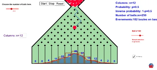
This example demonstrates the operation of a Galton board, illustrating probability distribution and statistical characteristics. Users can adjust parameters to observe ball distribution patterns under different settings. It utilizes commands such as Sequence, Point, Transform, and Vector for construction. Suitable for high school and above students to learn probability and statistics.
GeoGebra Commands & Parameters
Sequence(Sequence[(Reset * 0) + random(), i, 1, n], t, 1, m) → matrix1Sequence(Sequence[If[Element[Element[matrix1, t], i] < p, 0, 1], i, 1, n], t, 1, m) → matrix2Join({{(0, 0)}, Sequence[(Element[Element[matrix2, h + 1], i], 1 - Element[Element[matrix2, h + 1], i]), i, 1, n]}) → list3Sequence(Sum[list3, i], i, 1, n + 1) → list4Point(Ray[A, A + (1, 0)]) → BDilate(Rotate[B, 45°, A], 0.7071067811865475, A) → PVector(P, P + (A - P) / n) → uVector(P, P + (B - P) / n) → vSequence(Segment[P + (i * u), P + (i * u) + ((n - i) * v)], i, 0, n) → list1Sequence(Segment[P + (i * v), P + (i * v) + ((n - i) * u)], i, 0, n) → list2Point(Ray[A, A + (0, -1)]) → CTranslate(C, Vector[A, B]) → DSequence(Sum[Element[matrix2, i]], i, 0, h) → list6Sequence(-0.5 + i, i, 0, n + 1) → list7Frequency(list7, list6) → list8Sequence(A + (i * (B - A) / n), i, 1, n - 1) → list10Sequence(C + (i * (D - C) / n), i, 1, n) → list11Textfield(n) → inputBox1Sequence(((nCr[n, i] * p^(n - i)) * (1 - p)^(i)), i, 0, n) → list9Sum(Sequence[Polygon[C + ((((2 * i) - 2.8) * d), 0), C + ((((2 * i) - 1.2) * d), 0), C + ((((2 * i) - 1.2) * d), (Element[list9, i] * floor(abs(y(A) - y(C) - 1) / Max[list9]))), C + ((((2 * i) - 2.8) * d), (Element[list9, i] * floor(abs(y(A) - y(C) - 1) / Max[list9])))], i, 1, n + 1]) → fSum(Frequency[list7, Sequence[Sum[Element[matrix2, i]], i, 0, m]]) → gSequence(Polygon[C + ((((2 * i) - 2.8) * d), 0), C + ((((2 * i) - 1.2) * d), 0), C + ((((2 * i) - 1.2) * d), ((Element[list8, i] * 5) * f / 8 / g / d)), C + ((((2 * i) - 2.8) * d), ((Element[list8, i] * 5) * f / 8 / g / d))], i, 1, n + 2) → list14Sequence(PolyLine[C + ((((2 * i) - 2.8) * d), 0), C + ((((2 * i) - 2.8) * d), (Element[list9, i] * floor(abs(y(A) - y(C) - 1) / Max[list9]))), C + ((((2 * i) - 1.2) * d), (Element[list9, i] * floor(abs(y(A) - y(C) - 1) / Max[list9]))), C + ((((2 * i) - 1.2) * d), 0)], i, 1, n + 1) → list13Sequence(Segment[P + (x(Element[list4, i]) * v) + (y(Element[list4, i]) * u), P + (x(Element[list4, i + 1]) * v) + (y(Element[list4, i + 1]) * u)], i, 1, k) → list5Segment(C + (-0.8, 0), D + (0.8, 0)) → bSequence(A + (i * (B - A) / ((2 * n))), i, 1, (2 * n)) → liste1Sequence(C + (i * (D - C) / ((2 * n))), i, 1, (2 * n)) → liste2Sequence(Segment[Element[liste1, i], Element[liste2, i]], i, 1, Length[liste1], 2) → liste3Segment(E, F) → jSegment(EE, G) → lSequence(C + ((t - 1) * (D - C) / n) + (-0.1, ((5 * f / 8 / g / d) * Element[list8, t]) + 0.05), t, 1, n + 1) → liste4Sequence(Segment[Element[liste4, i], Element[liste4, i + 1]], i, 1, Length[liste4]) → liste5Circle(Ball, r) → qSequence(Sequence[Translate[H, Vector[(i * u) + (j * v)]], i, 0, n - j - 1], j, 0, n) → liste6Polygon(I, EE, E, J) → poly1, i_1, ee, e_1, j_1Segment(L, J) → sSegment(I, K) → tPolygon(E, EE, G, F) → poly2, e_2, ee_1, g_1, f_1Sequence(Circle[Element[liste7, i], r], i, 1, Length[liste7]) → liste8Sequence(Circle[Element[liste7, i], r], i, 1, Length[liste7]) → liste9Sequence(Text[Element[list8, t], C + ((t - 1) * (D - C) / n) + (-0.1, ((5 * f / 8 / g / d) * Element[list8, t]) + 0.325)], t, 1, n + 1) → list12
AI Drawing Prompt Reference
Draw a customizable Galton board experiment. At the top, pegs are arranged in a triangular grid. Balls drop from the top, randomly bounce left or right at each peg, and collect into vertical bins at the bottom. Below the bins, show both the theoretical probability distribution curve and the actual frequency histogram for comparison. Include sliders and an input box to adjust the number of balls, peg rows, and bias probability. Display paths of balls as polylines, bars for frequencies, and text labels for counts. The layout is clear for educational demonstration.
The prompt above was compiled from the original drawing commands and is for reference only.