
Continuous Probability Density Functions
Loading the math board and drawing, please wait…
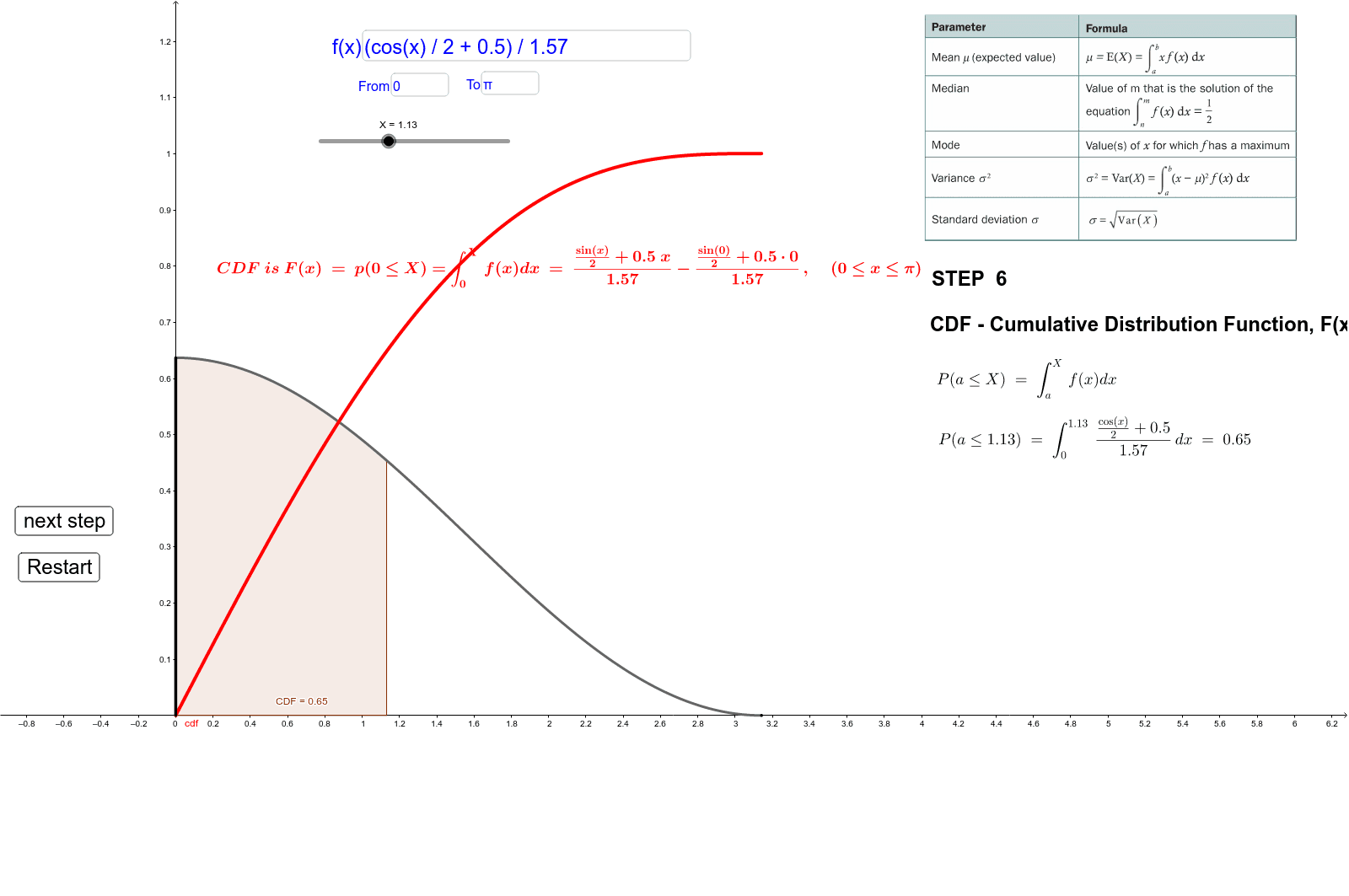
This example demonstrates how to graph continuous probability density functions and shows the integration process step by step. It uses commands like Integral, Segment, Sequence, and is suitable for IB Higher Level Mathematics.
GeoGebra Commands & Parameters
Integral(f) → intfIntegral(f, low, high) → Int1Segment(D, E) → bSegment(C, F) → cSequence(f(low + (k * (high - low) / 40)), k, 0, 40) → list1Max(list1) → maxvalueIntegral((x * f(x)), low, high) → meanSimplify(If[low ≤ x ≤ high, intf(x) - intf(0)]) → gSegment(I, H) → dIntegral(((x - mean)^(2) * f(x)), low, high) → VARTextfield(f) → InputBox1Textfield(low) → InputBox2Textfield(high) → InputBox3Integral(f, low, X) → CDFIntegral(f) → ggIntersect(g, a, (0.8312354302988411, 0.500000000003446)) → GOrthogonalLine(G, xAxis) → eIntersect(xAxis, e) → JSegment(G, J) → hMidpoint(G, J) → KSimplify(g) → p