
Continuity and Limits: Epsilon-Delta Visualization for Calculus
Loading the math board and drawing, please wait…
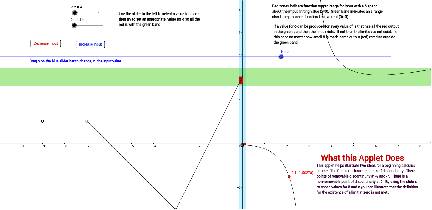
This GeoGebra applet illustrates foundational ideas for a beginning calculus course, focusing on points of discontinuity and removable discontinuities. It provides a dynamic visualization of limits and continuity using the epsilon-delta (ε-δ) framework. The construction relies on GeoGebra commands such as Function to plot the curve, Point to mark significant locations, OrthogonalLine and Line to construct local neighborhoods, Intersect to determine boundary points, Polygon to highlight relevant regions, and Text for annotations. Key objects include the function f, labeled points B through V, and the parameters ε and δ. The example is well suited for introductory calculus students and instructors who need an interactive tool to demonstrate how limits define continuity and how removable discontinuities appear graphically.
GeoGebra Commands & Parameters
Function(2 * x + 3, -3, 0) → gFunction((x + 9) * (x + 7) / ((x + 9) * (x + 7)), -10000, -7) → iPoint(g) → BFunction(1 / 4 * (x^(2) + 1) * x / (x * (x - 3)), 0, 10000) → fFunction((-x - 6) * (x + 7) / (x + 7), -7, -3) → hPoint(h) → EOrthogonalLine(K, xAxis) → aOrthogonalLine(L, xAxis) → cPolygon(M, N, O, P) → poly1, m, n, o, pOrthogonalLine(Q, yAxis) → dOrthogonalLine(R, yAxis) → ePolygon(S, T, U, V) → poly2, s, t, u, vIntersect(c, m) → AIntersect(c, m) → WIntersect(c, m) → ZLine(E, B) → kIntersect(k, c) → A_1OrthogonalLine(B, yAxis) → lOrthogonalLine(A_1, yAxis) → qIntersect(yAxis, q) → B_1Intersect(l, c) → C_1Polygon(A_1, B_1, B, C_1) → poly3, a_1, b_1, b_2, c_1Intersect(a, o) → D_1Intersect(a, o) → E_1Intersect(a, o) → F_1Intersect(a, o) → G_1OrthogonalLine(K, o) → rIntersect(a, o) → H_1Intersect(a, o) → I_1Intersect(a, o) → J_1Intersect(f, a, (0.15, -0.08969298245614034)) → K_1OrthogonalLine(K_1, yAxis) → d_1Intersect(yAxis, d_1) → L_1Polygon((0, 0), L_1, K_1, K) → poly5, e_1, f_1, g_1, h_1Text("Discontinuity at x = -9.") → text3Text("Discontinuity at x = -7.") → text4Text("Discontinuity at x = 0.") → text5Text("Removable") → text6Text("Removable") → text7Text("Nonremovable") → text8Text("Drag b on the blue slider bar to change, x, the input value.") → text10Text("What this Applet Does") → text12Text("Nonremovable") → text13Text("Discontinuity at x = 0.") → text14
AI Drawing Prompt Reference
Create a calculus teaching graph illustrating limits and continuity with an epsilon-delta visualization. The graph features a piecewise-defined curve with discontinuities at x = -9, x = -7, and x = 0, where the first two are removable and the last is nonremovable. Use perpendicular lines to construct local neighborhoods, determine boundary points via intersections, and highlight relevant regions with polygons. Label key points on the axes, add text annotations explaining each discontinuity type, and include a note prompting users to drag a slider to change the input value and observe the effect.
The prompt above was compiled from the original drawing commands and is for reference only.