Conic Sections in Polar Coordinates: Focus, Directrix, and Eccentricity

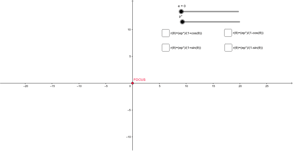
This GeoGebra example visualizes conic sections (ellipse, parabola, hyperbola) in polar coordinates using the unified equation r = ep/(1 ± e·cosθ) or r = ep/(1 ± e·sinθ). By adjusting the eccentricity e and focal parameter p via sliders, users can observe how the shape transitions among the three types of conics. The core mathematical concepts include polar equations, the focus-directrix definition of conics, eccentricity, and parametric curves. The construction uses the CurveCartesian command to plot the parametric curve, along with multiple objects (e, p, f, a, g, h, k, b, c, d, i, j, l, m, n, q, r, s) and a FOCUS object to mark the focus point. This interactive tool is suitable for high school or early college students studying analytic geometry, and for teachers demonstrating the unified polar representation of conic sections in classroom settings.