
Congruence Theorems: Dynamic Geometric Construction
Loading the math board and drawing, please wait…
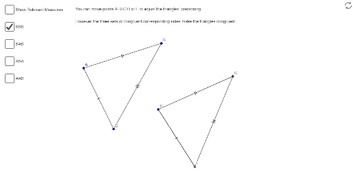
This GeoGebra example provides an interactive demonstration of triangle congruence theorems (such as SSS, SAS, ASA) through dynamic geometric construction. It visually shows how corresponding sides and angles of congruent triangles are equal, while also touching on related concepts like polygon perimeter and median values. The construction uses commands including Polygon, Circle, Point, Segment, Intersect, Angle, Rotate, and Ray to build auxiliary circles, intersection points, and rotated copies, creating multiple objects (A, B, C, poly1, D, F, G, E_1, etc.) that illustrate different congruence scenarios. A text object (text1) labels the final conclusion. This resource is ideal for middle or high school geometry classes, helping students grasp the conditions for triangle congruence and serving as a template for teachers to create their own dynamic demonstrations.
GeoGebra Commands & Parameters
Polygon(A, B, C) → poly1, c, a, bCircle(A, B) → dCircle(C, B) → eCircle(D, c) → fPoint(Circle[D, abs(b)]) → FSegment(D, F) → gCircle(F, a) → hIntersect(h, f) → E_1, G, ,Polygon(D, F, G) → poly2, g_1, d_1, f_1Segment(A, C) → iSegment(D, F) → jSegment(A, B) → kSegment(D, G) → lSegment(C, B) → mSegment(F, G) → nSegment(H, I) → pSegment(H, J) → qAngle(I, H, J) → αSegment(J, I) → rPoint(Circle[K, abs(q)]) → LSegment(K, L) → sRotate(K, (-α), L) → K'Angle(K', L, K) → βRay(L, K') → tCircle(L, p) → c_1Intersect(c_1, t) → M,Segment(M, K) → a_1Segment(L, M) → b_1Segment(N, O) → e_1Segment(P, N) → h_1Segment(P, O) → i_1Angle(O, N, P) → γAngle(P, O, N) → δPoint(Circle[Q, abs(e_1)]) → RSegment(Q, R) → j_1Rotate(R, γ, Q) → R'Angle(R, Q, R') → εRotate(Q, (-δ), R) → Q'Angle(Q', R, Q) → ζRay(Q, R') → k_1Ray(R, Q') → l_1Intersect(k_1, l_1) → SSegment(S, Q) → m_1Segment(S, R) → n_1Segment(T, U) → p_1Segment(U, V) → q_1Segment(V, T) → r_1Point(Circle[W, abs(p_1)]) → ZSegment(W, Z) → t_1Angle(T, U, V) → ηAngle(U, V, T) → θRotate(W, η, Z) → W'Angle(W, Z, W') → ιAngle(V, T, U) → κRotate(Z, (-κ), W) → Z'Angle(Z', W, Z) → λRay(Z, W') → a_2Ray(W, Z') → b_2Intersect(b_2, a_2) → ESegment(W, E) → c_2Segment(E, Z) → d_2Angle(Z, E, W) → μSegment(A, B) → e_2Segment(A, C) → f_2Segment(C, B) → h_2Segment(G, D) → i_2Segment(D, F) → j_2Segment(G, F) → k_2Segment(K, L) → l_2Segment(L, M) → m_2Segment(J, H) → n_2Segment(H, I) → p_2Angle(M, L, K) → νAngle(I, H, J) → ξSegment(N, O) → q_2Segment(Q, R) → r_2Angle(O, N, P) → οAngle(R, Q, S) → ρAngle(P, O, N) → σAngle(S, R, Q) → τSegment(U, T) → s_2Segment(Z, W) → t_2Angle(T, U, V) → υAngle(W, Z, E) → ϕAngle(U, V, T) → χAngle(Z, E, W) → ψ