
Conformal Mapping Demonstration
Loading the math board and drawing, please wait…
In collections
MATH3401 - Lectures
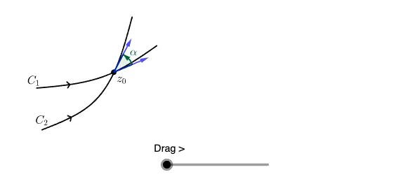
This example visually demonstrates the geometric properties of conformal mapping through dynamic graphics, illustrating how complex functions preserve angles and shapes. It involves core math concepts like complex numbers, function mapping, and transformation characteristics. GeoGebra commands and objects used include Spline, Point, Segment, Vector, Length, and Angle for construction. Suitable for high school and above learners to understand the visual representation and geometric meaning of complex functions.
GeoGebra Commands & Parameters
Spline({A, B, C}, 3) → aPoint(a) → GSpline({D, E, F}, 3) → bPoint(b) → HPoint(a) → IPoint(a) → JPoint(b) → KPoint(b) → LSegment(K, L) → gSegment(I, J) → jPoint(a) → MVector(M, N) → uVector(M, O) → vLength(u) → o1Length(v) → o2Angle(u, v) → αVector(P, (Q * t) + (N * (1 - t))) → wVector(P, (R * t) + (O * (1 - t))) → cLength(c) → o3Length(w) → o4Angle(w, c) → βSpline({(S * t) + (A * (1 - t)), (T * t) + (B * (1 - t)), (U * t) + (C * (1 - t))}, 3) → dSpline({(V * t) + (D * (1 - t)), (W * t) + (E * (1 - t)), (Z * t) + (F * (1 - t))}, 3) → ePoint(d) → A_1Point(d) → B_1Point(e) → C_1Point(e) → D_1Segment(A_1, B_1) → hSegment(C_1, D_1) → i
AI Drawing Prompt Reference
Draw a conformal mapping demonstration consisting of two smooth spline curves representing the domain and its image. Take points on each curve and draw segments connecting them to show corresponding relationships. Construct several vectors emanating from points on the curves to represent directions. Label the lengths of these vectors and the angles between them to visually demonstrate that conformal mapping preserves angles.
The prompt above was compiled from the original drawing commands and is for reference only.