
Cone and Linear Equations with 3D Geometric Transformations
Loading the math board and drawing, please wait…
In collections
Mapping Diagrams: From AB to C&DE, Resource
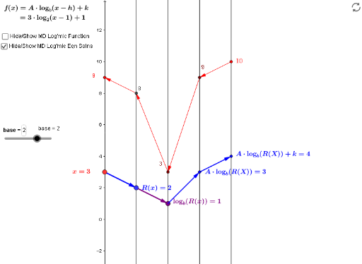
This example demonstrates the geometric transformations of a cone in three-dimensional space and its relationship with linear equations. The core math concepts involved include solid geometry, vector operations, linear equations, and three-dimensional coordinate transformations. The construction highlights the use of GeoGebra commands like Point, Vector, Textfield, and Sequence to create objects such as base points, vectors, text fields, and sequences, dynamically showcasing the transformation process. Suitable for high school and above students to understand the integration of spatial geometry and linear equations.
GeoGebra Commands & Parameters
Point(i) → KPoint(yAxis) → A_xVector(A_x, B_x) → uVector(B_x, C_x) → vTextfield(m) → inputBox1Textfield(s) → inputBoxfSequence(Vector[(6, m(core(R(i)))), (8, s(m(core(R(i)))))], i, 1, 5) → QuadgvlistSequence(Vector[(4, core(R(i))), (6, m(core(R(i))))], i, 1, 5) → QuadmvlistSequence(Vector[(0, i), (2, R(i))], i, 1, 5) → QuadRvlistSequence(Vector[(2, R(i)), (4, core(R(i)))], i, 1, 5) → QuadqvlistVector(K, s_{inv}D) → wVector(s_{inv}D, m_{invSinvD}) → zVector(m_{invSinvD}, q_{inv+}) → dVector(q_{inv+}, I) → h_1Sequence(Vector[(0, i), (2, m(i))], i, -2, 2) → LinmvlistSequence(Vector[(2, m(i)), (4, s(m(i)))], i, -2, 2) → LingvlistTextfield(h) → inputBox2Textfield(k) → inputBox3Textfield(A) → inputBox4Textfield(base) → inputBox5Vector(C_x, D_x) → fVector(D_x, E_x) → g