
Complex Mapping Diagram with Homotopy
Loading the math board and drawing, please wait…
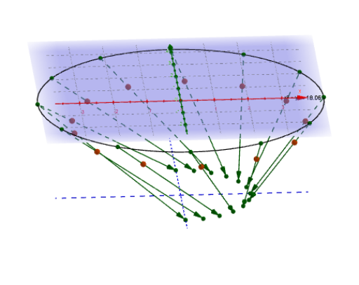
This example demonstrates a complex mapping diagram with homotopy, involving complex functions. Using GeoGebra commands such as Sequence, Zip, and CurveCartesian, the power function mapping is constructed. Suitable for high school mathematics education, particularly in complex numbers and functions.
GeoGebra Commands & Parameters
Sequence(t, t, t_0, t_2, dt) → t_*Zip((r * ℯ^((B * ί))), B, t_*) → z_*Zip((x(B), y(B), height_{image}), B, fz_*) → fpoint_*CurveCartesian((r * cos(t)), (r * sin(t)), height_{image}, t, 0, 6.283185307179586) → dTextfield(fz_*) → inputBox1Vector(z_#, f_{(z#).}) → wTextfield(f_{(z#)}) → inputBox2CurveCartesian(t, 0, height_{image}, t, -5, 5) → XhCurveCartesian(0, t, height_{image}, t, -5, 5) → YhTextfield(z_*) → inputBox3Sphere((0, 0, 4), 1) → RSZip(Segment[A, (0, 0, 5)], A, fpoint_*) → RS_vZip(Intersect[A, RS], A, RS_v) → RSpt_vIntersect(zAxis, RS, 2) → ASegment(A, f_{(z#).}) → fIntersect(f, RS) → P_∞, CZip(Vector[A, B], A, z_*, B, fpoint_*) → fvec_*Sequence(t, t, t_0 + dt, t_2 + dt, dt) → t_1Zip((r * ℯ^((B * ί))), B, t_1) → z_1Element(Euler_S, n + 1) → IntEstZip((real(Z), imaginary(Z), height_{image}), Z, Euler_S) → ESumSequence(Element[ESum, k], k, 1, n + 1) → ESum_nZip(Vector[A, B], A, z_*, B, ESum_n) → ESumV_nSequence(Element[dz_*, k], k, 1, n) → dz_nZip(Line[A, B], A, z_*, B, fpoint_*) → list1Zip(Intersect[h, Line[A, B]], A, z_*, B, fpoint_*) → list2