
Complex Linear Mapping Diagram II: f(z) = Az
Loading the math board and drawing, please wait…
In collections
Mapping Diagrams to Visualize Complex Analysis
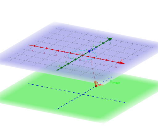
This example demonstrates the graphical transformation of the complex linear mapping f(z) = Az. Key mathematical concepts include complex numbers, linear mappings, and similar triangles. Using GeoGebra commands such as Sequence, Zip, and Textfield, the mapping of complex number z is constructed. Suitable for high school mathematics education and learning complex number transformations.
GeoGebra Commands & Parameters
Sequence((r * (cos(t) + (sin(t) * ί))), t, -3.141592653589793, 3.141592653589793, 0.5235987755982988) → z_*Zip(f(z), z, z_*) → fz_*Zip((x(z), y(z), height_{image}), z, fz_*) → fpoint_*Sequence(Vector[Element[z_*, j], Element[fpoint_*, j]], j, 1, 12) → fvec_*Textfield(fz_*) → inputBox1Vector(z_#, f_{(z#).}) → wTextfield(f_{(z#)}) → inputBox2CurveCartesian(t, 0, height_{image}, t, -5, 5) → XhCurveCartesian(0, t, height_{image}, t, -5, 5) → YhTextfield(z_*) → inputBox3Sequence(Line[Element[z_*, j], Element[fpoint_*, j]], j, 1, 12) → list1Intersect(zAxis, f_1) → VertexIntersect(xAxis, yAxis) → BPoint(xAxis) → CCircle(B, C) → pToPolar(A) → DCurveCartesian(((r * (1 - t / 3 + (ρ * t / 3))) * cos(Angle[z_#] + (t / 3 * Angle[A]))), ((r * (1 - t / 3 + (ρ * t / 3))) * sin(Angle[z_#] + (t / 3 * Angle[A]))), t, t, (-abs(z(Vertex))), abs(z(Vertex))) → jZip(CurveCartesian[((r * (1 - t / 3 + (ρ * t / 3))) * cos(Angle[w] + (t / 3 * Angle[A]))), ((r * (1 - t / 3 + (ρ * t / 3))) * sin(Angle[w] + (t / 3 * Angle[A]))), (-t), t, 0, abs(height_{image})], w, z_*) → fgeodesic_*If(z(Vertex) ≥ 0, Cone[(0, 0, height_{image}), Vertex, (r * ρ)], Cone[(0, 0, 0), Vertex, r]) → coneCircle((0, 0), 1) → unitCircle((0, 0), r) → cCurveCartesian(((r * ρ) * cos(t)), ((r * ρ) * sin(t)), height_{image}, t, 0, 6.28319) → d