Comparison of Poisson, Binomial, and Normal Distributions

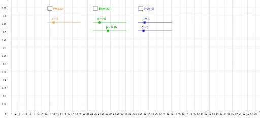
This interactive example provides a visual comparison between the Poisson, Binomial, and Normal distributions. It demonstrates the fundamental concepts of discrete and continuous probability distributions and illustrates how these distributions approximate one another under specific parameter conditions. The construction utilizes GeoGebra's specialized commands such as BinomialDist, Poisson, and Normal, with dynamic control provided by objects including $\lambda$, $n$, $p$, $\mu$, and $\sigma$. This tool is ideal for high school statistics students or undergraduate probability courses to visualize the convergence and differences between these key statistical models.