
Central Limit Theorem & Law of Large Numbers Demo
Loading the math board and drawing, please wait…
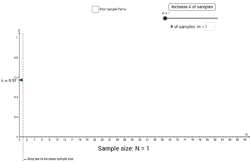
This example dynamically demonstrates the Central Limit Theorem and Law of Large Numbers through interactive visualizations. Key math concepts include probability distributions, sample means, normal distribution approximation, and statistical laws. GeoGebra commands and objects used in construction are Sequence, Line, Textfield, Point, Polygon, PolyLine, Segment, Histogram, Slider, etc. Ideal for high school and above students/teachers in mathematics and statistics education.
GeoGebra Commands & Parameters
Sequence(RandomUniform[0, 1, 50], i, 1, m) → UniformSampleSequence(Sequence[Sum[Element[UniformSample, i], j] / j, j, 1, 50], i, 1, m) → UniformMeansLine(A, B) → DragLineSequence(Point[{0, Element[UniformSample, 1, i]}], i, 1, floor(x(A))) → UniformPointsTextfield(m) → inputBox1Point({0.6, Element[UniformMeans, 1, floor(x(A))]}) → Sample1MeanSequence(Sequence[Sum[(Element[Transpose[UniformMeans], i] > (HistogramWidth * k)) ∧ (Element[Transpose[UniformMeans], i] < (HistogramWidth * (k + 1)))], k, 0, floor(1 / HistogramWidth)], i, 1, 50) → HistogramHeightsSequence(Polygon[{(HistogramxLocation, (HistogramWidth * (k - 1))), (HistogramxLocation + (Element[HistogramHeights, floor(x(A)), k] * HistogramMaxHeight / m), (HistogramWidth * (k - 1))), (HistogramxLocation + (Element[HistogramHeights, floor(x(A)), k] * HistogramMaxHeight / m), (HistogramWidth * k)), (HistogramxLocation, (HistogramWidth * k))}], k, 1, floor(1 / HistogramWidth)) → HistogramSequence(Sequence[Segment[(i - 1, Element[UniformMeans, j, i - 1]), (i, Element[UniformMeans, j, i])], j, 1, m], i, Max[2, floor(x(A)) - LengthOfLines], floor(x(A))) → UniformSampleLinesTextfield(LengthOfLines) → inputBox2Polygon(Corner[4], Corner[3], (0.8 * Corner[3]) + (0.2 * Corner[2]), (0.8 * Corner[4]) + (0.2 * Corner[1])) → poly1, b, c, d, ePolyLine((-0.2, 1.04), (0, 1.05), (0.2, 1.04)) → XaxisarrowPolyLine((HistogramxLocation - 0.2, 0.99), (HistogramxLocation, 1), (HistogramxLocation + 0.2, 0.99)) → histogramaxisarrowSegment(Sample1Mean, (HistogramxLocation, y(Sample1Mean))) → xbarguideline