
Central Limit Theorem: Distribution of Sample Means from a Skewed Population
Loading the math board and drawing, please wait…
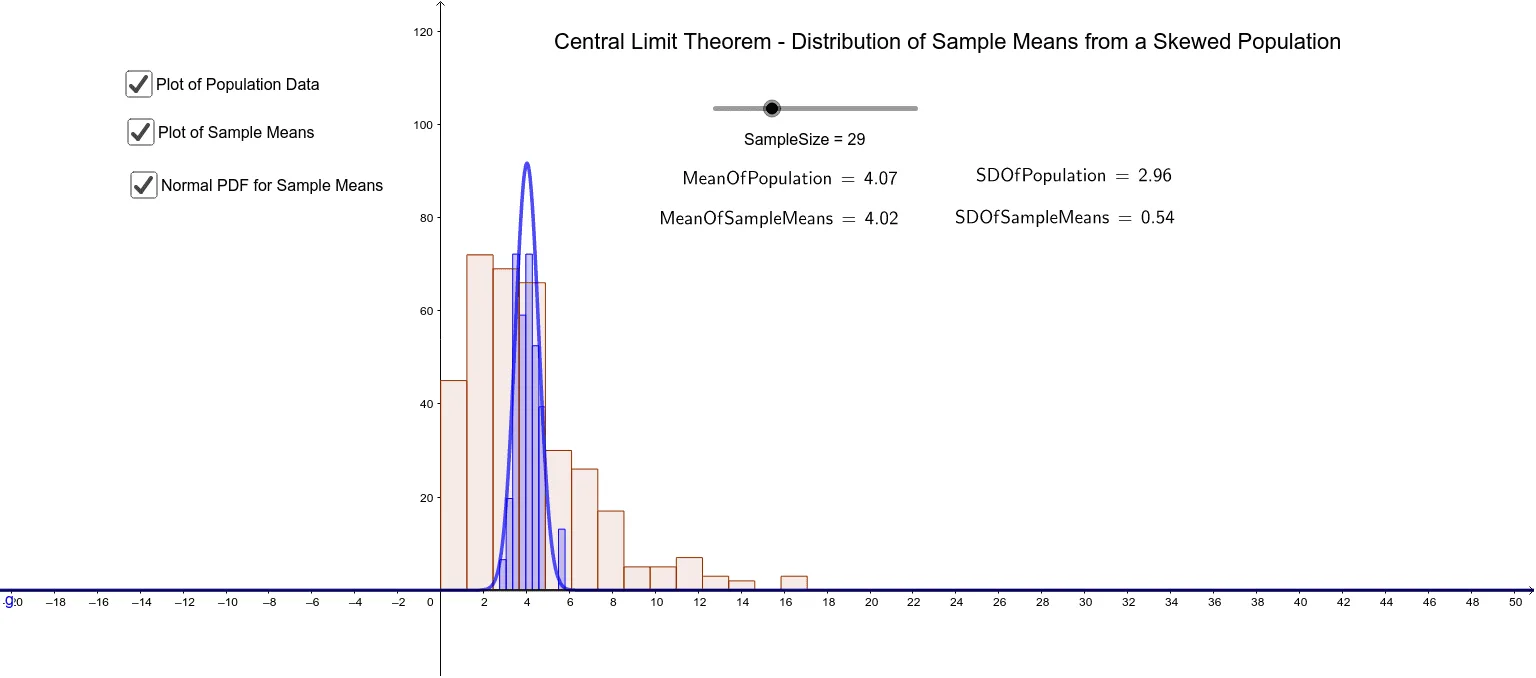
① This example dynamically demonstrates how the distribution of sample means approaches a normal distribution as sample size increases, even when the population is skewed. ② The core mathematical concept is the Central Limit Theorem (CLT), involving population distribution, sample means, standard deviation, histograms, and normal approximation. ③ Construction highlights: using GeoGebra commands such as Sample to draw samples from a skewed population, Mean and SD to compute statistics, and Histogram to plot the distribution of sample means; LaTeX is used for annotations, with objects like A350 storing intermediate results. ④ Suitable for high school to undergraduate statistics courses, particularly for visualizing sampling distributions and the CLT, and for exploring how sample size affects the shape of the distribution.
GeoGebra Commands & Parameters
Sample(list1, SampleSize) → F51Mean(F51) → G51Sample(list1, SampleSize) → F50Mean(F50) → G50Sample(list1, SampleSize) → F49Mean(F49) → G49Sample(list1, SampleSize) → F48Mean(F48) → G48Sample(list1, SampleSize) → F47Mean(F47) → G47Sample(list1, SampleSize) → F46Mean(F46) → G46Sample(list1, SampleSize) → F45Mean(F45) → G45Sample(list1, SampleSize) → F44Mean(F44) → G44Sample(list1, SampleSize) → F43Mean(F43) → G43Sample(list1, SampleSize) → F42Mean(F42) → G42Sample(list1, SampleSize) → F41Mean(F41) → G41Sample(list1, SampleSize) → F40Mean(F40) → G40Sample(list1, SampleSize) → F39Mean(F39) → G39Sample(list1, SampleSize) → F38Mean(F38) → G38Sample(list1, SampleSize) → F37Mean(F37) → G37Sample(list1, SampleSize) → F36Mean(F36) → G36Sample(list1, SampleSize) → F35Mean(F35) → G35Sample(list1, SampleSize) → F34Mean(F34) → G34Sample(list1, SampleSize) → F33Mean(F33) → G33Sample(list1, SampleSize) → F32Mean(F32) → G32Sample(list1, SampleSize) → F31Mean(F31) → G31Sample(list1, SampleSize) → F30Mean(F30) → G30Sample(list1, SampleSize) → F29Mean(F29) → G29Sample(list1, SampleSize) → F28Mean(F28) → G28Sample(list1, SampleSize) → F27Mean(F27) → G27Sample(list1, SampleSize) → F26Mean(F26) → G26Sample(list1, SampleSize) → F25Mean(F25) → G25Sample(list1, SampleSize) → F24Mean(F24) → G24Sample(list1, SampleSize) → F23Mean(F23) → G23Sample(list1, SampleSize) → F22Mean(F22) → G22Sample(list1, SampleSize) → F21Mean(F21) → G21Sample(list1, SampleSize) → F20Mean(F20) → G20Sample(list1, SampleSize) → F19Mean(F19) → G19Sample(list1, SampleSize) → F18Mean(F18) → G18Sample(list1, SampleSize) → F17Mean(F17) → G17Sample(list1, SampleSize) → F16Mean(F16) → G16Sample(list1, SampleSize) → F15Mean(F15) → G15Sample(list1, SampleSize) → F14Mean(F14) → G14Sample(list1, SampleSize) → F13Mean(F13) → G13Sample(list1, SampleSize) → F12Mean(F12) → G12Sample(list1, SampleSize) → F11Mean(F11) → G11Sample(list1, SampleSize) → F10Mean(F10) → G10Sample(list1, SampleSize) → F9Mean(F9) → G9Sample(list1, SampleSize) → F8Mean(F8) → G8Sample(list1, SampleSize) → F7Mean(F7) → G7Sample(list1, SampleSize) → F6Mean(F6) → G6Sample(list1, SampleSize) → F5Mean(F5) → G5Sample(list1, SampleSize) → F4Mean(F4) → G4Sample(list1, SampleSize) → F3Mean(F3) → G3Sample(list1, SampleSize) → F2Mean(F2) → G2Sample(list1, SampleSize) → F1Mean(F1) → G1Mean(list5) → H2SD(list5) → H3LaTeX(MeanOfSampleMeans, true, true) → text5LaTeX(SDOfSampleMeans, true, true) → text6Histogram(list4, list5, true, 2) → hMean(list1) → MeanOfPopulationSD(list1) → D2Histogram(list2, list1, false, 2) → aLaTeX(MeanOfPopulation, true, true) → text1SD(list1) → SDOfPopulationLaTeX(SDOfPopulation, true, true) → text2
AI Drawing Prompt Reference
Create an example showing how the distribution of sample means approaches a normal distribution as the sample size increases, even when the population is skewed. Start by drawing multiple samples from a skewed population, calculate the mean of each sample, and then plot the histogram of these means to observe the shape change.
The prompt above was compiled from the original drawing commands and is for reference only.