
Center of Mass of Hemisphere and Cone
Loading the math board and drawing, please wait…
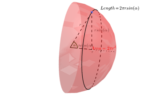
This example demonstrates the calculation and visualization of the center of mass for a hemisphere-cone composite solid. Key math concepts include solid geometry, center of mass computation, and integral applications. Construction highlights involve GeoGebra commands like Intersect, Surface, Point, Segment, Circle, CurveCartesian, Angle, and Cone. Suitable for high school students and math enthusiasts studying solid geometry and center of mass calculations.
GeoGebra Commands & Parameters
Intersect(yAxis, zAxis) → BSurface((-sin(v)), (sin(u) * cos(v)), (cos(u) * cos(v)), u, 0, 6.28319, v, -3.14159, 0) → aPoint(Segment[(0, 0, 0), (1, 0, 0)]) → ASegment((0, 0, 0), (1, 0, 0)) → bCircle(b, C) → cSegment(C, A) → dSegment(C, B) → eSurface((-sin(v)), (sin(u) * cos(v)), (cos(u) * cos(v)), u, 0, 6.28319, v, -3.14159, 0) → gSurface((x(A) * (-sin(v))), ((x(A) * sin(u)) * cos(v)), ((x(A) * cos(u)) * cos(v)), u, 0, 6.28319, v, -3.14159, 0) → hCurveCartesian(cos(u), 0, sin(u), u, -1.5707963267948966, 1.5707963267948966) → iPoint(i) → DAngle((1, 0, 0), B, D) → αSegment(B, D) → jCircle(b, D) → kSegment(D, E) → lSegment(E, B) → mPoint(Ray[B, A]) → FPoint(Ray[F, Vector[(0, 0, 1)]]) → GSegment(B, F) → nSegment(F, G) → pCone(F, B, p) → o, q, rPoint(n) → HCircle(n, I) → sSegment(H, I) → t