
Boxplots and Outliers
Loading the math board and drawing, please wait…
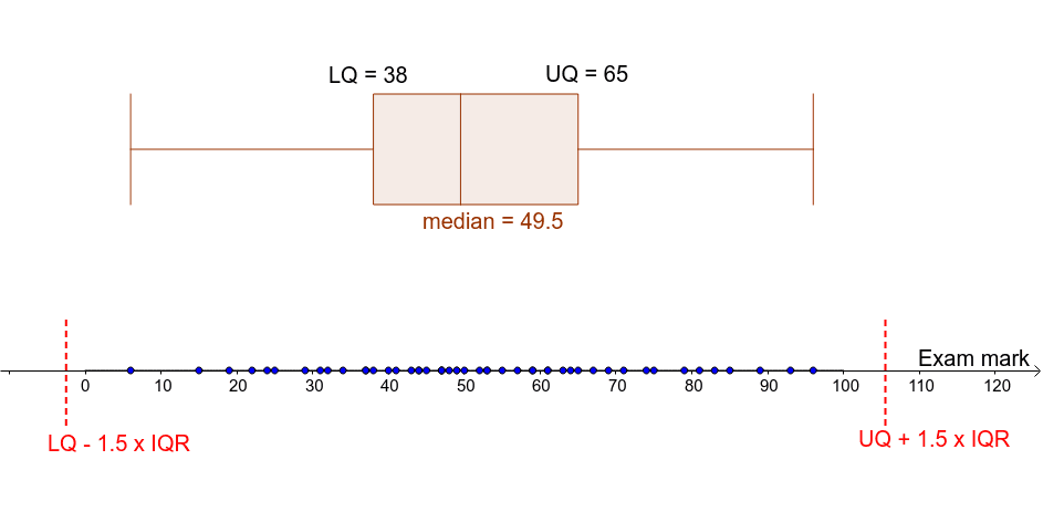
This example demonstrates the construction of boxplots and the identification of outliers. A boxplot is a statistical chart that shows the distribution of a dataset, including the median, quartiles, and outliers. Using GeoGebra commands, you can easily create a boxplot and analyze data distribution. The core mathematical concepts involved include statistics such as quartiles, median, and outliers. Construction highlights include the use of Function, Point, BoxPlot, Q1, Q3, Segment, and other commands. Suitable for middle school and above students to learn data statistics and analysis.
GeoGebra Commands & Parameters
Function(0, 0, 100) → fPoint(f) → A2Point(f) → A3Point(f) → A4Point(f) → A5Point(f) → A6Point(f) → A7Point(f) → A8Point(f) → A9Point(f) → A10Point(f) → A11Point(f) → A12Point(f) → A13Point(f) → A14Point(f) → A15Point(f) → A16Point(f) → A17Point(f) → A18Point(f) → A19Point(f) → A20Point(f) → A21Point(f) → A22Point(f) → A23Point(f) → A24Point(f) → A25Point(f) → A26Point(f) → A27Point(f) → A28Point(f) → A29Point(f) → A30Point(f) → A31Point(f) → A32Point(f) → A33Point(f) → A34Point(f) → A35Point(f) → A36Point(f) → A37Point(f) → A38Point(f) → A39Point(f) → A40Point(f) → A41Point(f) → A42Point(f) → A43Point(f) → A44Point(f) → A45Point(f) → A46Point(f) → A47Point(f) → A48Point(f) → A49Point(f) → A50Point(f) → A1BoxPlot(4, 1, L_1) → medianQ1(L_1) → q_1Q3(L_1) → q_3Segment((p, -1), (p, 1)) → bSegment((r, -1), (r, 1)) → cIf((B1 < r) ∨ (B1 > p), 1, 0) → C1If((B2 < r) ∨ (B2 > p), 1, 0) → C2If((B3 < r) ∨ (B3 > p), 1, 0) → C3If((B4 < r) ∨ (B4 > p), 1, 0) → C4If((B5 < r) ∨ (B5 > p), 1, 0) → C5If((B6 < r) ∨ (B6 > p), 1, 0) → C6If((B7 < r) ∨ (B7 > p), 1, 0) → C7If((B8 < r) ∨ (B8 > p), 1, 0) → C8If((B9 < r) ∨ (B9 > p), 1, 0) → C9If((B10 < r) ∨ (B10 > p), 1, 0) → C10If((B11 < r) ∨ (B11 > p), 1, 0) → C11If((B12 < r) ∨ (B12 > p), 1, 0) → C12If((B13 < r) ∨ (B13 > p), 1, 0) → C13If((B14 < r) ∨ (B14 > p), 1, 0) → C14If((B15 < r) ∨ (B15 > p), 1, 0) → C15If((B16 < r) ∨ (B16 > p), 1, 0) → C16If((B17 < r) ∨ (B17 > p), 1, 0) → C17If((B18 < r) ∨ (B18 > p), 1, 0) → C18If((B19 < r) ∨ (B19 > p), 1, 0) → C19If((B20 < r) ∨ (B20 > p), 1, 0) → C20If((B21 < r) ∨ (B21 > p), 1, 0) → C21If((B22 < r) ∨ (B22 > p), 1, 0) → C22If((B23 < r) ∨ (B23 > p), 1, 0) → C23If((B24 < r) ∨ (B24 > p), 1, 0) → C24If((B25 < r) ∨ (B25 > p), 1, 0) → C25If((B26 < r) ∨ (B26 > p), 1, 0) → C26If((B27 < r) ∨ (B27 > p), 1, 0) → C27If((B28 < r) ∨ (B28 > p), 1, 0) → C28If((B29 < r) ∨ (B29 > p), 1, 0) → C29If((B30 < r) ∨ (B30 > p), 1, 0) → C30If((B31 < r) ∨ (B31 > p), 1, 0) → C31If((B32 < r) ∨ (B32 > p), 1, 0) → C32If((B33 < r) ∨ (B33 > p), 1, 0) → C33If((B34 < r) ∨ (B34 > p), 1, 0) → C34If((B35 < r) ∨ (B35 > p), 1, 0) → C35If((B36 < r) ∨ (B36 > p), 1, 0) → C36If((B37 < r) ∨ (B37 > p), 1, 0) → C37If((B38 < r) ∨ (B38 > p), 1, 0) → C38If((B39 < r) ∨ (B39 > p), 1, 0) → C39If((B40 < r) ∨ (B40 > p), 1, 0) → C40If((B41 < r) ∨ (B41 > p), 1, 0) → C41If((B42 < r) ∨ (B42 > p), 1, 0) → C42If((B43 < r) ∨ (B43 > p), 1, 0) → C43If((B44 < r) ∨ (B44 > p), 1, 0) → C44If((B45 < r) ∨ (B45 > p), 1, 0) → C45If((B46 < r) ∨ (B46 > p), 1, 0) → C46If((B47 < r) ∨ (B47 > p), 1, 0) → C47If((B48 < r) ∨ (B48 > p), 1, 0) → C48If((B49 < r) ∨ (B49 > p), 1, 0) → C49If((B50 < r) ∨ (B50 > p), 1, 0) → C50
AI Drawing Prompt Reference
Create a boxplot to display data distribution and identify outliers. Start by drawing a horizontal line as a data baseline, then place multiple random data points along this line to represent a sample dataset. Calculate the lower quartile, upper quartile, and median from these points, and draw a box spanning from the lower to the upper quartile, with a line inside marking the median. Extend two whiskers from the box ends to the maximum and minimum non-outlier values. Finally, mark any points beyond the whiskers as outliers. The chart should clearly show the data's central tendency, spread, and outliers.
The prompt above was compiled from the original drawing commands and is for reference only.