
Bivariate Normal Distribution
Loading the math board and drawing, please wait…
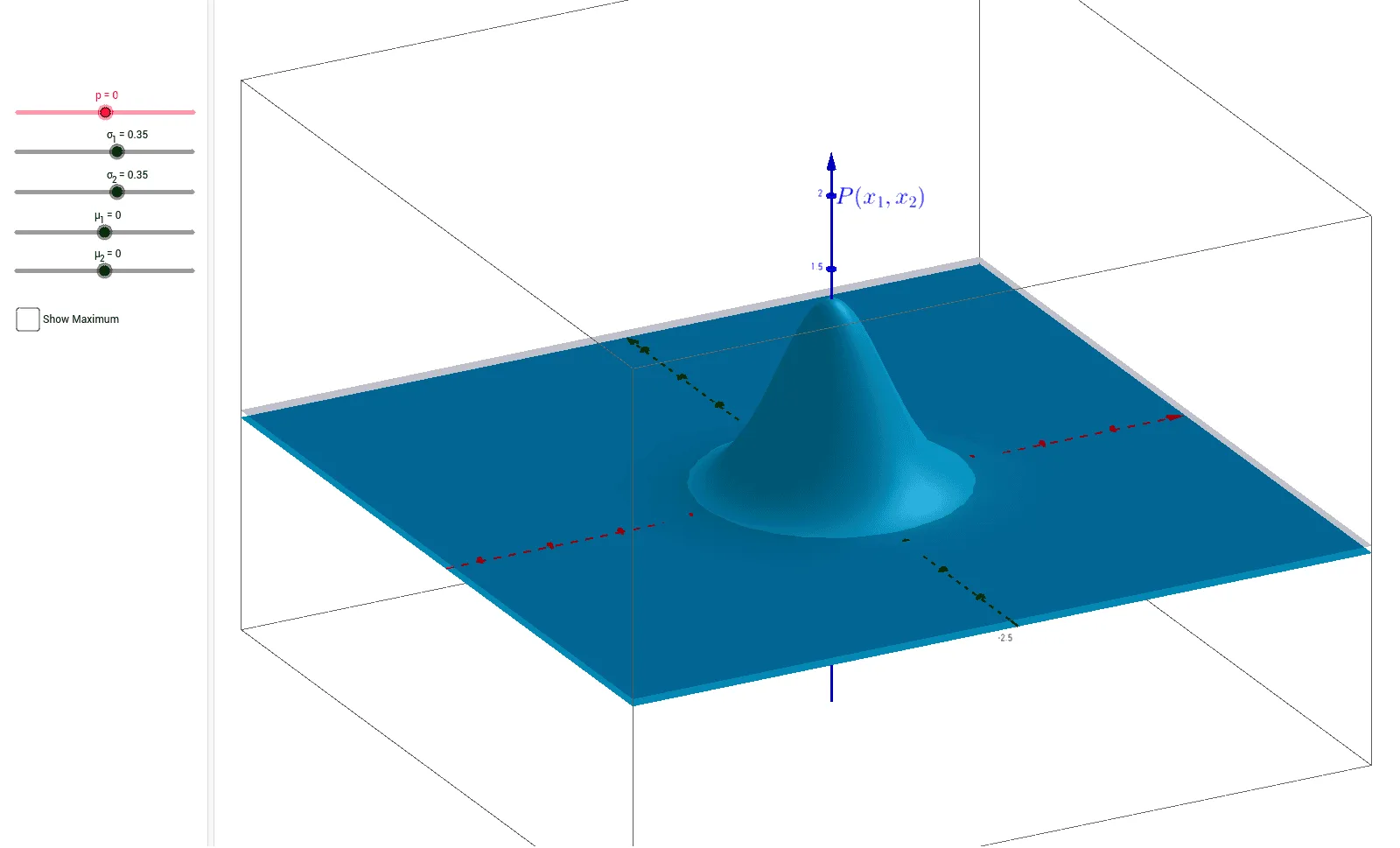
This example demonstrates the graphical representation and properties of the bivariate normal distribution. It involves core mathematical concepts such as normal distribution, probability density function, and parameter adjustments (mean, variance). The construction uses GeoGebra commands and objects like p, σ_1, σ_2, a, Coeff, μ_1, μ_2, Denom, d, b, Maximum, text1, Max, text2, text3, text4 for parameterized graphing and display. Suitable for high school students and above, particularly those interested in multivariate data analysis and statistics.
GeoGebra Commands & Parameters
Numeric p(0.0)Numeric σ_1(0.35)Numeric σ_2(0.35)a:1 / ((2 * π))1 / (((((2 * π) * σ_1) * σ_2) * sqrt(1 - p^(2))))Numeric μ_1(0.0)Numeric μ_2(0.0)-1 / ((2 * (1 - p^(2))))d(x, y) = (Coeff * ℯ^((Denom * ((x - μ_1)^(2) / σ_1^(2) - (((2 * p) * (x - μ_1)) * (y - μ_2) / ((σ_1 * σ_2))) + (y - μ_2)^(2) / σ_2^(2)))))b:z = 0.05(μ_1, μ_2, Coeff)Boolean Max(false)