
Binomial Distribution: B(n,p) with PDF and CDF
Loading the math board and drawing, please wait…
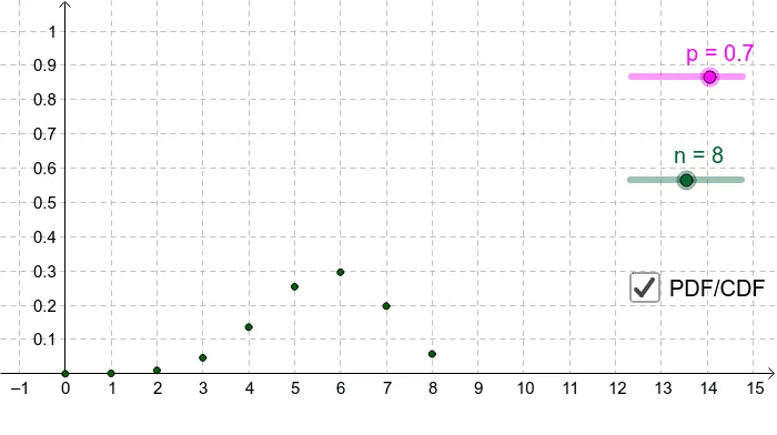
This example demonstrates the probability mass function (PMF) and cumulative distribution function (CDF) of a binomial distribution. Users can adjust parameters n and p to observe changes in the distribution. Key mathematical concepts include binomial distribution, probability and statistics. GeoGebra commands used include Sequence and Segment.
GeoGebra Commands & Parameters
Sequence(k - 1, k, 1, N) → list1Sequence(Binomial[n, k] * p^(k) * (1 - p)^(n - k), k, 0, n) → list2Sequence((Element[list1, k], Element[list2, k]), k, 1, N) → list3Sequence(Sum[Take[list2, 1, k]], k, 1, N) → list4Sequence((Element[list1, k], Element[list4, k]), k, 1, N) → list5Sequence((Element[list1, k + 1], Element[list4, k]), k, 1, N) → list6Sequence(Segment[Element[list5, k], Element[list6, k]], k, 1, N - 1) → list7Segment((Element[list1, 1] - 5, 0), (Element[list1, 1], 0)) → aSegment((Element[list1, Length[list1]], 1), (Element[list1, Length[list1]] + 5, 1)) → b
AI Drawing Prompt Reference
Draw a binomial distribution B(n,p) with its probability mass function (PMF) and cumulative distribution function (CDF). Adjust n and p to observe changes in the distribution. First, draw the PMF as a bar chart, then draw the CDF as a line graph, and finally connect the bar chart and the line graph with segments to form the step-like CDF.
The prompt above was compiled from the original drawing commands and is for reference only.