
Binomial and Normal Approximation
Loading the math board and drawing, please wait…
In collections
MA336
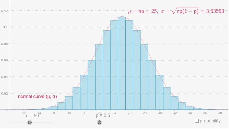
This example demonstrates the approximation of the binomial distribution using the normal distribution. It involves key concepts in probability and statistics, constructed using GeoGebra commands such as Segment, Point, BinomialDist, Normal, etc. Suitable for high school and above students or teachers to understand the relationship between different probability distributions.
GeoGebra Commands & Parameters
Segment(A, B) → ePoint(e) → CSegment(C, B) → gBinomialDist(n, p) → aNormal(mean, sd, x) → fMax(f, 0, 100) → maxSequence(Segment[(-10, i), (110, i)], i, 0.02, 0.5, 0.02) → list1Point(g) → DIntegral(f, x(C), x(D)) → pr_NBinomialDist(n, p, x(C), true) → cBinomialDist(n, p, x(D), true) → d
AI Drawing Prompt Reference
Draw a graph showing the approximation of the binomial distribution by the normal distribution, including a horizontal line segment and a vertical line segment forming a rectangle, with different colored areas inside representing the binomial and normal distributions, and the area under the normal distribution curve and the probability between two points for the binomial distribution, finally adding thin lines for the normal distribution curve and the cumulative distribution function lines of the binomial distribution.
The prompt above was compiled from the original drawing commands and is for reference only.