
Bernstein Polynomials
Loading the math board and drawing, please wait…
In collections
Mathematics of Computer Graphics
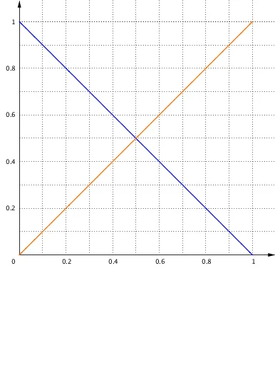
This example demonstrates the graph and properties of Bernstein polynomials, which are important tools in approximation theory for polynomial interpolation. By adjusting parameters, observe the shape changes of the polynomial. The construction uses commands like Sequence, Text, Integral, suitable for high school mathematics education and learning.
GeoGebra Commands & Parameters
Text(Simplify[((Binomial[n - 1, i - 1] * x^(i - 1)) * (1 - x)^(n - i))]) → Tform0Length(Tform0) → lä0Take(Tform0, (läg0 * zl_0) + 1, lä0) → Liste0RSequence(Take[Tform0, ((i - 1) * zl_0) + 1, (i * zl_0)], i, 1, läg0) → Liste0Text(Simplify[((Binomial[n - 1, i] * x^(i)) * (1 - x)^(n - i - 1))]) → TTerm1Length(TTerm1) → lä1Take(TTerm1, (läg1 * zl_1) + 1, lä1) → Liste1RSequence(Take[TTerm1, ((i - 1) * zl_1) + 1, (i * zl_1)], i, 1, läg1) → Liste1Text(Simplify[((Binomial[n, i] * x^(i)) * (1 - x)^(n - i))]) → Tform2Length(Tform2) → lä2Take(Tform2, (läg2 * zl_2) + 1, lä2) → Liste2RSequence(Take[Tform2, ((i - 1) * zl_2) + 1, (i * zl_2)], i, 1, läg2) → Liste2Sequence(((Binomial[n, i] * t_1^(i)) * (1 - t_1)^(n - i)), i, 0, n) → BernsteinPJoin({{0}, BernsteinP}) → H_2Sequence(Sum[Take[H_2, 1, j]], j, 1, n + 2) → H_4Point(Segment[T_0, T_{10}]) → V_1Point(Segment[T_0, T_{10}]) → V_2Sequence(Polygon[T_0 + ((scl * Element[H_4, i + 1]), 0), T_0 + ((scl * Element[H_4, i + 2]), 0), T_0 + ((scl * Element[H_4, i + 2]), scl_2), T_0 + ((scl * Element[H_4, i + 1]), scl_2)], i, 0, n, 2) → H_5Sequence(Polygon[T_0 + ((scl * Element[H_4, i + 1]), 0), T_0 + ((scl * Element[H_4, i + 2]), 0), T_0 + ((scl * Element[H_4, i + 2]), scl_2), T_0 + ((scl * Element[H_4, i + 1]), scl_2)], i, 1, n + 1, 2) → H_6Sequence((t_1, Element[BernsteinP, i + 1]), i, 0, n) → QSequence(If[0 ≤ x ≤ 1, ((Binomial[n, i] * x^(i)) * (1 - x)^(n - i))], i, 0, n, 2) → Bernstein1Sequence(If[0 ≤ x ≤ 1, ((Binomial[n, i] * x^(i)) * (1 - x)^(n - i))], i, 1, n, 2) → Bernstein2TextToUnicode(Tform2) → TfrmuniDegree(p) → mSequence(i / m, i, 0, m) → PktpSequence(((Binomial[m, i] * x^(i)) * (1 - x)^(m - i)), i, 0, m) → BasisTextfield(p) → EF1Sequence(p(j / m), j, 0, m) → LexpSequence(Text[Element[Lexp, j + 1]] + "\cdot " + (Text[((Binomial[m, j] * x^(j)) * (1 - x))]) + "^{" + (Text[m - j]) + "}", j, 0, m) → LBZIntegral(f, 0, 1) → ifCorner(1, 1) → Ep_1Corner(1, 2) → Ep_2Corner(1, 3) → Ep_3Corner(1, 4) → Ep_4
AI Drawing Prompt Reference
Draw the graph of Bernstein polynomials to demonstrate their function curves and properties, observing shape changes by adjusting parameters. First, plot the function curve of the polynomial, then construct a stepped shape using multiple polygons to represent the polynomial's behavior over the interval [0,1]. Finally, label key points and parameters for clarity.
The prompt above was compiled from the original drawing commands and is for reference only.