
Basic Trig Functions from the Unit Circle (Degrees)
Loading the math board and drawing, please wait…
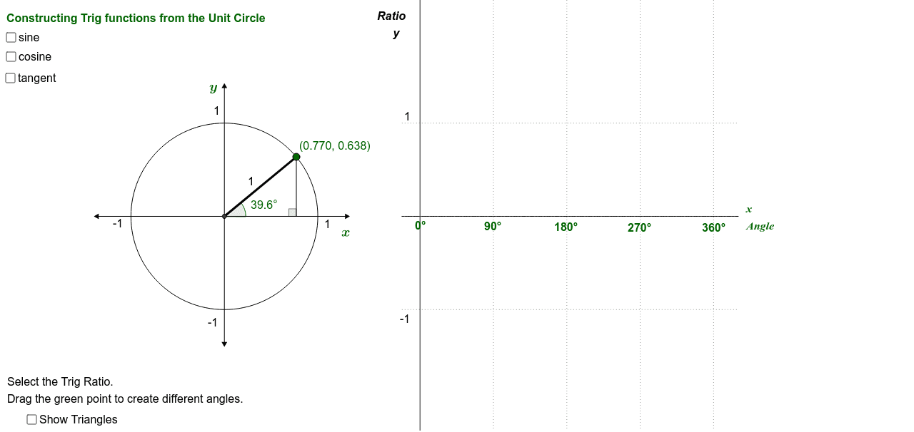
This GeoGebra example visually demonstrates the definitions and geometric meanings of the basic trigonometric functions (sine, cosine, and tangent) using the unit circle in degree mode. It illustrates how the coordinates of a point moving on the unit circle correspond to the values of sinα, cosα, and tanα, and how these values are projected onto their respective function graphs. Key mathematical concepts include the unit circle, trigonometric ratios, angle measurement in degrees, and the relationship between circular motion and periodic functions. The construction employs GeoGebra commands such as Circle, Point, Intersect, OrthogonalLine, Segment, Ray, Angle, Function, and Slider to create an interactive diagram where dragging the point or adjusting the angle slider updates the trigonometric values and graphs in real time. This resource is ideal for high school students learning trigonometry, teachers demonstrating the unit circle approach, and anyone seeking an intuitive visual foundation for understanding sine, cosine, and tangent functions.
GeoGebra Commands & Parameters
Intersect(xAxis, yAxis) → AFunction(0, 1.9, 5.5) → gPoint(g) → QPoint(yAxis) → BCircle(A, B) → cPoint(c) → DTangent(D, c) → e,Intersect(e, yAxis) → FIntersect(xAxis, e) → ESegment(F, E) → lSegment(E, A) → mIntersect(m, l) → OIntersect(c, xAxis, 2) → CSegment(A, C) → dOrthogonalLine(D, d) → fIntersect(f, m) → HSegment(A, H) → cosαAngle(Q, A, D) → αSegment(A, D) → bSegment(D, E) → tanαSegment(D, H) → sinαOrthogonalLine(D, sinα) → iFunction(sin((2 * (x - (2 * 3.14 / 3)))), 2.09, 5.24) → sineαIntersect(sineα, h, (2.439250960476847, 0.6379515420040821)) → IFunction(tan((2 * (x - (2 * 3.14 / 3)))), 2.09, 5.24) → tangentαIntersect(tangentα, h, (2.439250960476847, 0.8284261815090247)) → JFunction(cos((2 * (x - (2 * 3.14 / 3)))), 2.09, 5.24) → cosineαIntersect(cosineα, h, (2.439250960476847, 0.770076509221398)) → KSegment(H, D) → jSegment(A, F) → kIntersect(j, m) → NIntersect(k, l) → PFunction(1, 1.9, 5.5) → pFunction(-1, 1.9, 5.5) → qPoint(c) → RSegment(C, R) → aSegment(A, H) → g_1Segment(D, H) → h_1Segment(A, E) → j_1Angle(A, D, E) → βRay(D, F) → i_1Ray(D, E) → l_1Intersect(c, a) → G, LOrthogonalLine(I, xAxis) → d_1Intersect(g, xAxis, 1) → MIntersect(g, xAxis, 1) → SIntersect(g, xAxis, 1) → TIntersect(g, d_1) → USegment(I, U) → e_1OrthogonalLine(K, xAxis) → k_1Intersect(k_1, xAxis) → VSegment(K, V) → m_1OrthogonalLine(J, xAxis) → n_1Intersect(n_1, xAxis) → WSegment(J, W) → p_1Point(yAxis) → ZPoint(yAxis) → A_1Segment(Z, A_1) → q_1Point(xAxis) → B_1Point(xAxis) → C_1Segment(B_1, C_1) → r_1OrthogonalLine(D, r_1) → c_1Intersect(g, r_1, 1) → D_1Intersect(c_1, r_1) → E_1Segment(D, E_1) → s_1Angle(D, E_1, A) → γ
AI Drawing Prompt Reference
Draw a unit circle with a point on it representing angle α. Show the line from the origin to the point, and its projections onto the x-axis and y-axis. Illustrate the sine, cosine, and tangent lines, and project them onto their respective sine, cosine, and tangent curves. Include an angle slider that updates all visuals and values in real time when moved.
The prompt above was compiled from the original drawing commands and is for reference only.