Balancing Equations

Loading the math board and drawing, please wait…

2016-08-22 23:25

Function Coordinate Geometry

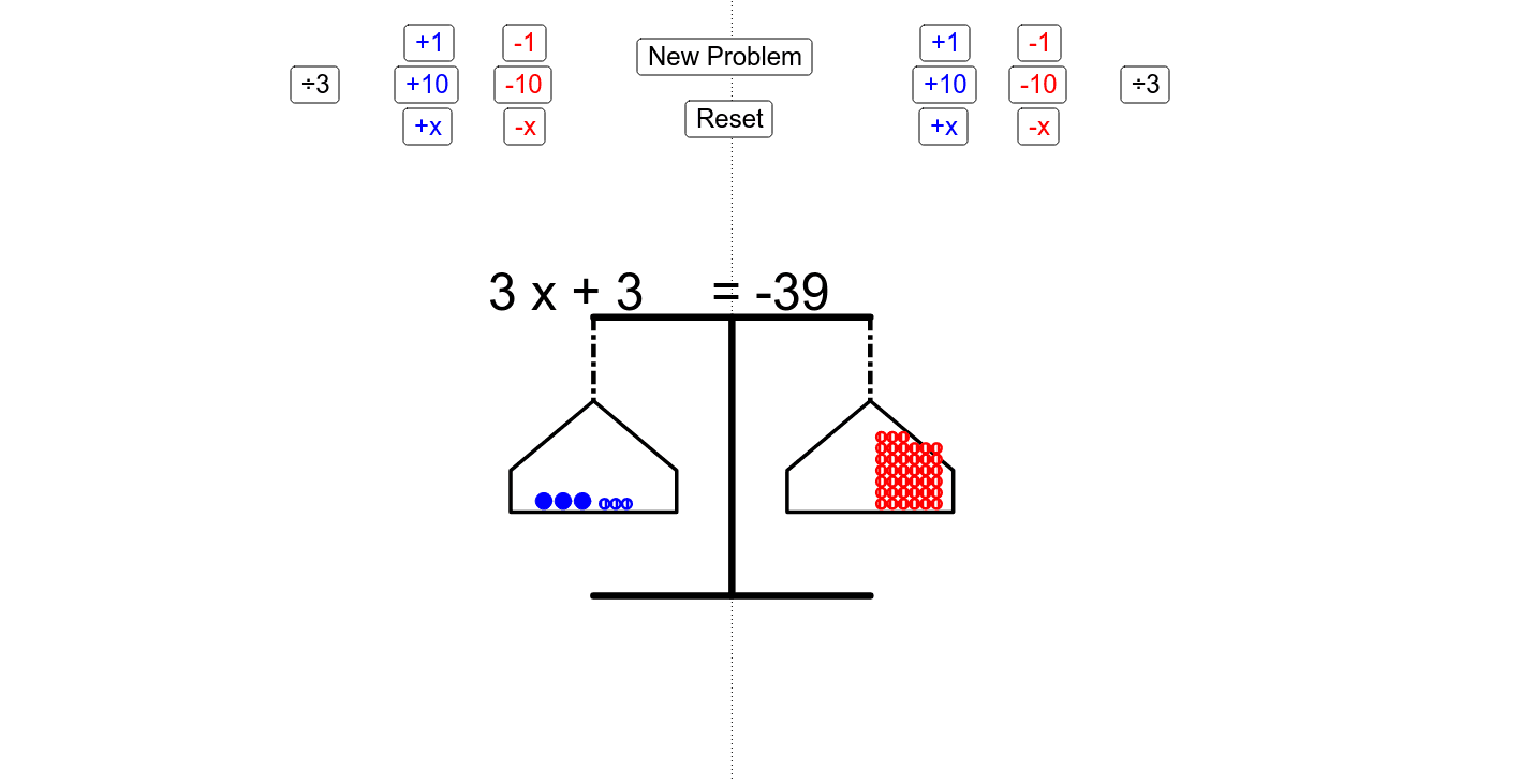
This example demonstrates the principle of equation balancing through dynamic interaction. It involves core math concepts like equation balancing, coordinate geometry, function graphing, and dynamic geometric transformations. Construction highlights include commands like Sequence, Segment, Point, and objects such as animate_d and balance_x for dynamic balance visualization, along with Slider Animation for parameter adjustment. Suitable for high school mathematics teaching to understand equation balancing and function properties.

GeoGebra Commands & Parameters

Sequence(Segment[Element[balanceCorners, k], Element[balanceCorners, k] + (0, (-3))], k, 1, 2) → balanceChains
Segment(Element[balanceCorners, 1], Element[balanceCorners, 2]) → balancePost_1
Segment((-5, -10), (5, -10)) → balancePost_2
Segment((0, 0), (0, -10)) → balancePost_3
Point(e) → A
Point(e) → B
Point(e) → C
Sequence(Polygon[Element[balanceCorners, k] + (0, (-3)), Element[balanceCorners, k] + (3, (-5.5)), Element[balanceCorners, k] + (3, (-7)), Element[balanceCorners, k] + ((-3), (-7)), Element[balanceCorners, k] + ((-3), (-5.5))], k, 1, 2) → balanceTrays
Sequence(Circle[(x(Element[balanceCorners, 1]) - 0.4 - (0.7 * Mod[k, 4]), (0.7 * floor(k / 4)) + y(Element[balanceCorners, 1]) - 6.6), 0.3], k, 0, abs(a) - 1) → LeftXBeads
Sequence(Circle[(x(Element[balanceCorners, 1]) + 0.4 + (0.4 * Mod[k, 6]), (0.4 * floor(k / 6)) + y(Element[balanceCorners, 1]) - 6.7), 0.175], k, 0, abs(b) - 1) → LeftNumberBeads
Sequence(Circle[(x(Element[balanceCorners, 2]) + 0.4 + (0.4 * Mod[k, 6]), (0.4 * floor(k / 6)) + y(Element[balanceCorners, 2]) - 6.7), 0.175], k, 0, abs(d) - 1) → RightNumberBeads
Sequence(Circle[(x(Element[balanceCorners, 2]) - 0.4 - (0.7 * Mod[k, 4]), (0.7 * floor(k / 4)) + y(Element[balanceCorners, 2]) - 6.6), 0.3], k, 0, abs(c) - 1) → RightXBeads