
Area Under the Curve: Visualizing Upper, Lower, and Midpoint Riemann Sums
Loading the math board and drawing, please wait…
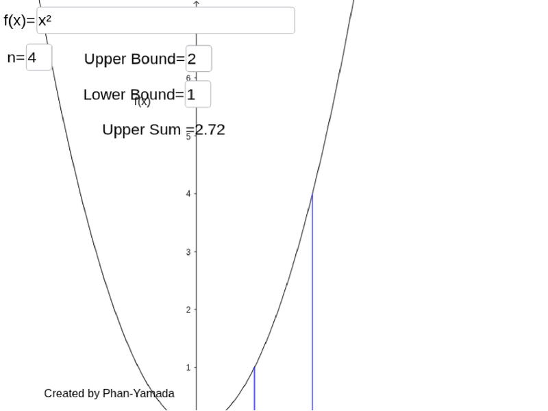
① This GeoGebra example dynamically visualizes the area between a function curve and the x-axis, approximating it using upper, lower, and midpoint Riemann sums. ② Core mathematical concepts include the geometric interpretation of definite integrals, Riemann sums, limits, and exponential functions. ③ Construction details: The commands UpperSum and LowerSum generate upper and lower sums; Sequence and Segment create partition points and rectangles; Textfield and input boxes allow interactive adjustment of interval and number of subdivisions; midpoint sequences (seqmidpt, seqfmidpt) and their sum (sumofmidpt) are displayed, along with multiple text objects (text1–text6) for labeling. ④ Suitable for high school to early college calculus courses, this example helps students grasp the approximation of integrals and explore function behavior and area computation.
GeoGebra Commands & Parameters
UpperSum(f, x(A), x(B), n) → UpperLowerSum(f, x(A), x(B), n) → LowerTextfield(f) → inputBox1Textfield(n) → inputBox2Textfield(b) → inputBox4Textfield(a) → inputBox3Sequence(Midpoint[(a + (i * (b - a) / n), 0), (a + ((i + 1) * (b - a) / n), 0)], i, 0, n - 1) → seqmidpt, {(1.125, 0), (1.375, 0), (1.625, 0), (1.875, 0)}Sequence((a + (i * (b - a) / ((2 * n))), f(a + (i * (b - a) / ((2 * n))))), i, 1, (2 * n), 2) → seqfmidpt, {(1.125, 1.265625), (1.375, 1.890625), (1.625, 2.640625), (1.875, 3.515625)}Sequence(Segment[Element[seqmidpt, i], Element[seqfmidpt, i]], i, 1, n) → seqmidseg, {1.265625, 1.890625, 2.640625, 3.515625}Sequence(f(a + (i * (b - a) / ((2 * n)))), i, 1, (2 * n), 2) → seqfmidptonly, {1.265625, 1.890625, 2.640625, 3.515625}Sequence(a + (i * (b - a) / n), i, 0, n) → seqpt, {1, 1.25, 1.5, 1.75, 2}Sequence(Polygon[(Element[seqpt, i], 0), (Element[seqpt, i], Element[seqfmidptonly, i]), (Element[seqpt, i + 1], Element[seqfmidptonly, i]), (Element[seqpt, i + 1], 0)], i, 1, n) → list1, {0.31640625, 0.47265625, 0.66015625, 0.87890625}Segment((a, 0), (a, f(a))) → gSegment((b, 0), (b, f(b))) → h
AI Drawing Prompt Reference
Draw a function curve and the area between it and the x-axis, approximated by upper, lower, and midpoint Riemann sums. Divide the interval into equal subintervals, and for each subinterval draw three rectangles: one using the maximum function value (upper sum), one using the minimum (lower sum), and one using the midpoint value. Use distinct colors for each type. Show the partition points, vertical segments at interval ends, and the function values at midpoints. Include input fields to adjust the function, interval endpoints, and number of subdivisions. Display the approximate area values for each sum. The layout should clearly illustrate how rectangles approximate the area under the curve.
The prompt above was compiled from the original drawing commands and is for reference only.