Area Under Polar Curves Visualization

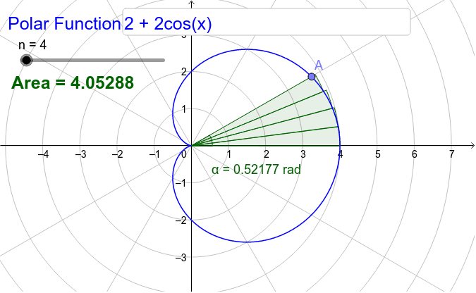
This GeoGebra example dynamically demonstrates how to compute the area enclosed by a polar curve. It visualizes the process of dividing the region between the curve and the polar axis into small sectors as the polar angle sweeps from a start to an end value, then summing these sector areas to approximate the true area. The core mathematical concept is the polar-coordinate definite integral, specifically the area formula A = 1/2 ∫ r(θ)² dθ, along with the ideas of limits and Riemann sums. Construction highlights: the CurveCartesian command is used to plot the polar curve in parametric form; Sequence and Sum commands generate and accumulate a series of small sector areas; an Angle object marks the polar angle range; a Slider controls the number of subdivisions n to show convergence. Interactive components such as Point, Textfield, and InputBox allow users to modify parameters. This example is suitable for advanced high school or introductory college calculus students to grasp the geometric meaning and numerical approximation of the polar area formula, and it also serves as an effective classroom demonstration tool.