Another Road Up a Mountain

Loading the math board and drawing, please wait…

2016-04-07 05:15

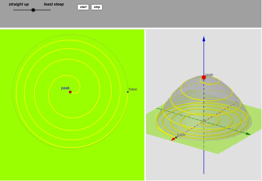
This example demonstrates the graphical representation of roads and paths on a mountain in three-dimensional space. The core mathematical concepts involved include piecewise functions, polynomial functions, LCM and GCD, geometric distribution, and normal distribution. Construction highlights extracted from the GeoGebra command summary include Circle, CurveCartesian, Cone, Rotate, and Point commands/objects. Suitable for high school and above, this can be used for teaching demonstrations or student exploration in spatial geometry and function graphing.

GeoGebra Commands & Parameters

Circle(A, R) → c
CurveCartesian((t^(0.5) * cos((f * t))), (t^(0.5) * sin((f * t))), t, 0, R^(2)) → a
Cone(A, C, R) → b, d, e
Rotate(a, ((-R^(2)) * f)) → a'
Point(a') → G
CurveCartesian(X(t), Y(t), Z(t), t, 0, R^(2)) → k
Rotate(k, ((-R^(2)) * f)) → k'

AI Drawing Prompt Reference

Draw a mountain in 3D space as a cone with its apex at the top and a circular base at the bottom. From the apex, a spiral road winds down along the cone's surface, generated by rotating a planar curve defined by parametric equations involving square root and trigonometric functions. Mark a point on this rotated curve to indicate a specific location on the road. Additionally, include another spatial curve representing a second path, also rotated to lie on the cone's surface. Show the overall spatial relationship among the mountain, the two paths, and the key point.

The prompt above was compiled from the original drawing commands and is for reference only.