
Analyzing Relationship Between Class Size and Test Scores
Loading the math board and drawing, please wait…
In collections
UCSS Secondary Math I Unit 4 Lesson 3
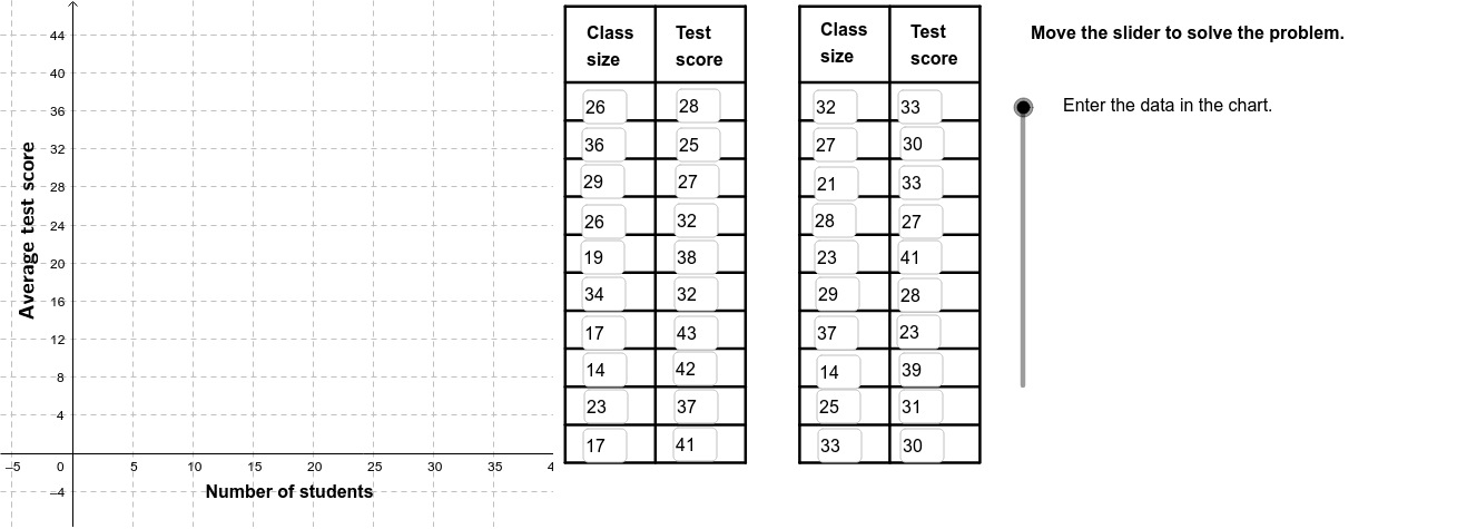
This example demonstrates how to analyze the relationship between class size and standardized test scores using a scatter plot. Key math concepts include correlation (PMCC), linear regression (FitLineY), and data visualization (Scatter Plot). The construction involves commands like FitLineY for linear fitting, PMCC for correlation calculation, Textfield for displaying text, If for conditional logic, Polygon for creating polygons, Sequence for generating sequences, Segment for drawing segments, and RotateText for rotating text. It is suitable for high school mathematics education, particularly for introductory statistics and data analysis courses.
GeoGebra Commands & Parameters
FitLineY(PointList1) → LineFitPMCC(PointList1) → CorCoeffTextfield(A2) → InA2Textfield(A3) → InA3Textfield(A4) → InA4Textfield(A5) → InA5Textfield(A6) → InA6Textfield(A7) → InA7Textfield(A8) → InA8Textfield(A9) → InA9Textfield(A10) → InA10Textfield(A11) → InA11Textfield(A12) → InA12Textfield(A13) → InA13Textfield(A14) → InA14Textfield(A15) → InA15Textfield(A16) → InA16Textfield(A17) → InA17Textfield(A18) → InA18Textfield(A19) → InA19Textfield(A20) → InA20Textfield(A21) → InA21Textfield(B2) → InB2Textfield(B3) → InB3Textfield(B4) → InB4Textfield(B5) → InB5Textfield(B6) → InB6Textfield(B7) → InB7Textfield(B8) → InB8Textfield(B9) → InB9Textfield(B10) → InB10Textfield(B11) → InB11Textfield(B12) → InB12Textfield(B13) → InB13Textfield(B14) → InB14Textfield(B15) → InB15Textfield(B16) → InB16Textfield(B17) → InB17Textfield(B18) → InB18Textfield(B19) → InB19Textfield(B20) → InB20Textfield(B21) → InB21If(CorVisible, "Hide Correlation Coefficient", "Show Correlation Coefficient") → CorButtonIf(LineVisible, "Hide Best Fit Line", "Show Best Fit Line") → LineButtonPolygon((40, y(Corner[1])), Corner[2], Corner[3], (40, y(Corner[4]))) → poly1, a, b, c, dSequence(Segment[(41, -1 + (4 * i)), (56, -1 + (4 * i))], i, 0, 10) → Linesh1Sequence(Segment[(41 + (7.5 * i), -1), (41 + (7.5 * i), 47)], i, 0, 2) → Linesv1Sequence(Segment[(60.5 + (7.5 * i), -1), (60.5 + (7.5 * i), 47)], i, 0, 2) → Linesv2Sequence(Segment[(60.5, -1 + (4 * i)), (75.4, -1 + (4 * i))], i, 0, 10) → Linesh2Segment((41, 47), (56, 47)) → top1Segment((60.5, 47), (75.5, 47)) → top2RotateText("Average test score", 90*°) → SideLegend
AI Drawing Prompt Reference
Create a scatter plot to show the relationship between class size and standardized test scores. First, plot the scatter points, then add the best fit line and correlation coefficient. Use text boxes to display the correlation coefficient and the equation of the line. Click buttons to toggle the visibility of the correlation coefficient and the best fit line. Finally, add grid lines and axis labels to make the chart clearer.
The prompt above was compiled from the original drawing commands and is for reference only.