
3D Velocity Field Particles Demo
Loading the math board and drawing, please wait…
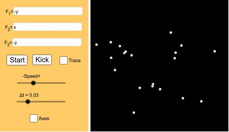
This example demonstrates the dynamic distribution and variation of particle velocity fields in 3D space. Core math concepts include vector fields, 3D coordinates, velocity functions, and trigonometry. Construction involves using Textfield commands to set parameters, with objects like Speed, g, f, A1-A20, B1-B16 to build the vector field model. Suitable for high school students and math enthusiasts studying vector calculus and spatial geometry applications.
GeoGebra Commands & Parameters
Textfield(f) → InputBox1Textfield(g) → InputBox2Textfield(h) → InputBox3SelectedIndex(Options) → IndexOptions
AI Drawing Prompt Reference
Create a 3D visualization of a dynamic velocity field with particles. The scene shows a volumetric grid of glowing particles, each with an arrow indicating velocity direction and magnitude, varying smoothly across space. Include three input boxes for adjusting the velocity field functions and a dropdown menu to switch between different field modes. Use semi-transparent particles and colored arrows against a dark background, with particles moving along curved paths to illustrate the field's spatial variation and flow.
The prompt above was compiled from the original drawing commands and is for reference only.