
3D Function
Loading the math board and drawing, please wait…
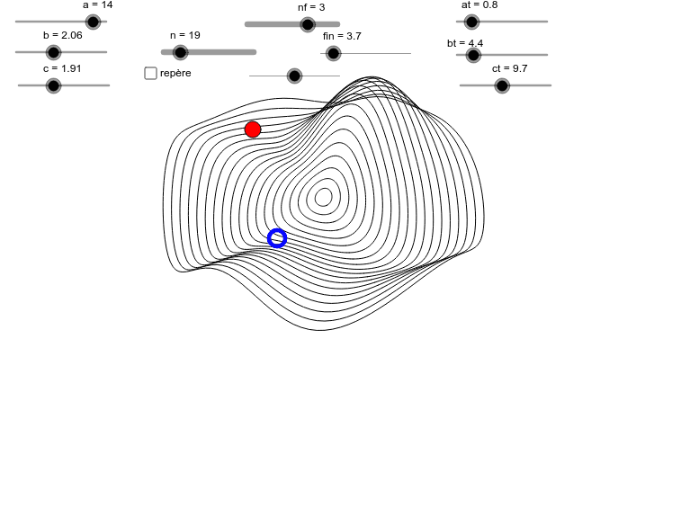
This example demonstrates a 3D function graph. Key mathematical concepts include functions, parametric equations, and coordinate geometry. By adjusting parameters with sliders, you can observe changes in the function graph. GeoGebra commands used include Element, Sequence, Vector, and Line. Suitable for high school and above students to learn about 3D functions and parametric equations.
GeoGebra Commands & Parameters
Element(listef, nf) → fSequence(CurveCartesian[((kxx * i) * cos(t)) + ((kyx * i) * sin(t)), ((kxy * i) * cos(t)) + ((kyy * i) * sin(t)) + (kzy * f((i * cos(t)), (i * sin(t)))), t, 0, 6.28319], i, fin / n, fin, fin / n) → couVector((0, 0), I) → vxVector((0, 0), J) → vyVector((0, 0), K) → vzLine((0, 0), I) → dxLine((0, 0), J) → dyLine((0, 0), K) → dz
AI Drawing Prompt Reference
Draw a 3D function graph with x, y, and z axes and their corresponding unit vectors vx, vy, and vz. Adjust parameters to observe changes in the graph. Use parametric equations to represent the curve, where the x and y coordinates are kxx*i*cos(t) + kxy*i*sin(t) and kyx*i*cos(t) + kyy*i*sin(t) + kzy*f(i*cos(t), i*sin(t)), respectively, with t ranging from 0 to 2π.
The prompt above was compiled from the original drawing commands and is for reference only.