2D Steiner Theorem: Invariance of the Sum of Squared Distances

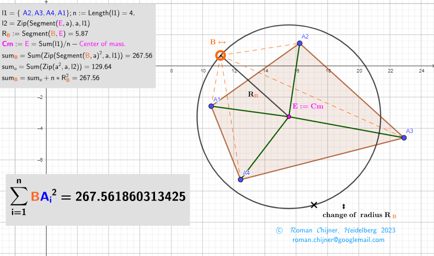
This GeoGebra example demonstrates a 2D invariance phenomenon: when a moving point is constrained by a geometric setup, the sum of squared distances to selected reference points (linked to the centroid/barycenter structure) remains constant. The key ideas are Steiner’s theorem about decomposing sums of squared distances, the centroid/barycenter, and geometric constructions involving circles, parallelogram-type configurations, and circumcircle relationships. Construction-wise, it uses Polygon to create the main polygonal configuration (e.g., A1–A4), Point and Circle to define key points and circles (such as I, q1, B), Segment/Length to measure relevant distances, and Sum to aggregate squared-distance terms (e.g., sum_o, sum_B) while Text labels the invariant quantities (txt, text1, text3). The example is suited for students learning centroid methods, proof intuition for distance-squared identities, and dynamic geometry exploration in secondary competitions and advanced geometry instruction.