
兔子种群增长散点图分析
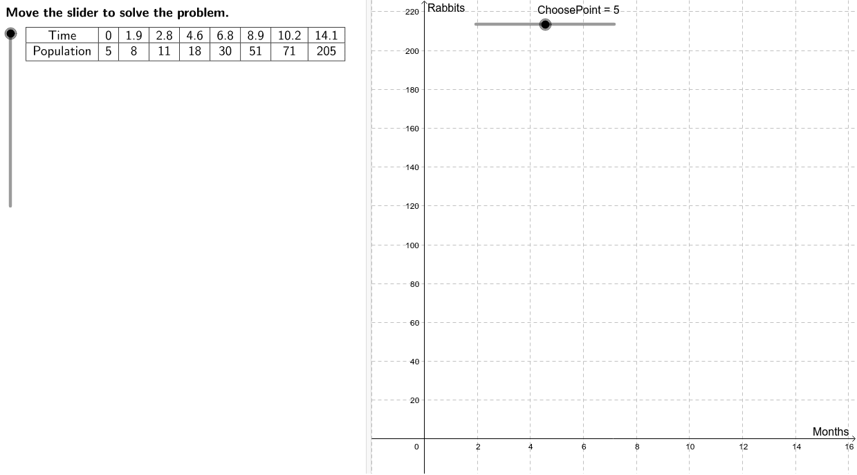
几何画板及绘图内容加载中,请稍等……
①本范例通过散点图演示兔子种群随时间的变化趋势;②涉及核心数学概念包括数据分析、函数拟合、微积分中的导数与积分;③构造摘要中使用了LaTeX、表格、滑块、数据缩放等GeoGebra命令与对象;④适合高中数学教学,用于讲解数据可视化与函数建模。
GeoGebra 命令及参数
LaTeX(steps) → counterLaTeX("\text{Move the slider to solve the problem.}") → text0LaTeX("\text{Use the buttons below to return to the original}\cr\text{problem or randomly generate a similar practice}\cr\text{problem.}") → RandomizationTextCorner(1) → ACorner(3) → BCell(2, ChoosePoint) → n_{model}Cell(1, ChoosePoint) → t_{model}LaTeX("\text{Create a scatter plot of the data.}") → text1LaTeX("\text{Let }\textcolor{#000099}{x}\text{ represent the number of months and }\textcolor{#000099}{y}\cr\text{represent the rabbit population.}") → text2LaTeX("\text{Write an equation that describes the function.}") → text3LaTeX("\text{The data appears to follow an exponential curve in}\cr\text{the form }\textcolor{#006633}{y = a b^x}\text{, for which }\textcolor{#006633}{a}\text{ is the y-intercept of}\cr\text{the graph.}") → text4LaTeX((((("\text{From the data table, it can be seen that the}\cr\text{y-intercept is }\textcolor{#006633}{(0, " * n_{start}) * ")}\text{. Therefore, }\textcolor{#006633}{a = ") * n_{start}) * "}.")) → text5LaTeX((((((("\text{Choose a second point from the data table such}\cr\text{as }\textcolor{#006633}{(" * t_{model}) * ", ") * n_{model}) * " )}\text{. Substitute these }\textcolor{#006633}{x}\text{ and }\textcolor{#006633}{y}\text{ values as}\cr\text{well as the value of }\textcolor{#006633}{a=") * n_{start}) * "}\text{ into the general form }\cr\textcolor{#006633}{y = a b^x}\text{ and solve for }\textcolor{#006633}{b}.")) → text6LaTeX("\text{Use the ChoosePoint slider to see how the}\cr\text{equation modeling the data depends on which}\cr\text{data point is used to solve for }\textcolor{#006633}{b}.") → text10LaTeX("\text{Create a residual plot to check if the function model}\cr\text{is a good fit for the situation.}") → text11LaTeX("\text{Plot the residuals and determine if the function is}\cr\text{a good fit for the data.}") → text18LaTeX("\text{Use the function to predict the rabbit population}\cr\text{after 16 months.}") → text20LaTeX((("\text{After 16 months, there will be approximately }\cr" * n_{16}) * "\text{ rabbits, assuming their population continues}\cr\text{to grow at this rate.}")) → text23Max({E1, E2, E3, E4, E5, E6, E7, E8}) → maxResidMin({E1, E2, E3, E4, E5, E6, E7, E8}) → minResidMax((maxResid * 1.1), maxResid + 1) → ymaxRTableText({{LaTeX["Time"], LaTeX[A1], LaTeX[A2], LaTeX[A3], LaTeX[A4], LaTeX[A5], LaTeX[A6], LaTeX[A7], LaTeX[A8]}, {LaTeX["Population"], LaTeX[B1], LaTeX[B2], LaTeX[B3], LaTeX[B4], LaTeX[B5], LaTeX[B6], LaTeX[B7], LaTeX[B8]}}, "c_|") → ProblemTableText({{LaTeX["x"], LaTeX[(((("\textcolor{#006633}{y_0=" * n_{start}) * "(") * b) * ")^x}")]}, {LaTeX[A1], LaTeX[D1]}, {LaTeX[A2], LaTeX[D2]}, {LaTeX[A3], LaTeX[D3]}, {LaTeX[A4], LaTeX[D4]}, {LaTeX[A5], LaTeX[D5]}, {LaTeX[A6], LaTeX[D6]}, {LaTeX[A7], LaTeX[D7]}, {LaTeX[A8], LaTeX[D8]}}, "c_|") → text15LaTeX("\text{Create a table of each x-value and its}\cr\text{corresponding model y-value (}\textcolor{#006633}{y_0}\text{). Round }\textcolor{#006633}{y_0}\text{ to}\cr\text{the nearest integer since it is not possible to have}\cr\text{a fraction of a rabbit.}") → text14LaTeX("\text{Find the difference between the observed value}\cr\text{and calculated value for each value of }\textcolor{#006633}{x}\text{. This}\cr\text{difference, }\textcolor{#006633}{y – y_0}\text{, is the residual.}") → text16TableText({{LaTeX["\textcolor{#006633}{x}"], LaTeX["\text{residual (}\textcolor{#006633}{y-y_0}\text{)}"]}, {LaTeX[A1], LaTeX[((((B1 * "-") * D1) * "=") * E1)]}, {LaTeX[A2], LaTeX[((((B2 * "-") * D2) * "=") * E2)]}, {LaTeX[A3], LaTeX[((((B3 * "-") * D3) * "=") * E3)]}, {LaTeX[A4], LaTeX[((((B4 * "-") * D4) * "=") * E4)]}, {LaTeX[A5], LaTeX[((((B5 * "-") * D5) * "=") * E5)]}, {LaTeX[A6], LaTeX[((((B6 * "-") * D6) * "=") * E6)]}, {LaTeX[A7], LaTeX[((((B7 * "-") * D7) * "=") * E7)]}, {LaTeX[A8], LaTeX[((((B8 * "-") * D8) * "=") * E8)]}}, "c_|") → text17LaTeX((((("\text{Since the points appear to be spread out}\cr\text{randomly, }\textcolor{#006633}{y_0 = " * n_{start}) * "(") * b) * ")^x}\text{ is a good fit for the}\cr\text{data.}")) → text19LaTeX("\text{Substitute for }\textcolor{#006633}{a}\text{ and }\textcolor{#006633}{b}\text{ in the general form }\textcolor{#006633}{y=ab^x}\text{.}\cr\text{Since }\textcolor{#006633}{y}\text{ is used for the observed values of the}\cr\text{population, use }\textcolor{#006633}{y_0}\text{ in this equation modeling the}\cr\text{data.}") → text8LaTeX((((("\textcolor{#006633}{y_0 = " * n_{start}) * "(") * b) * ")^x}")) → text9LaTeX((((("\text{The residual is the difference between the observed}\cr\text{value and the estimated value using the function }\cr\textcolor{#006633}{y_0 = " * n_{start}) * "(") * b) * ")^x}.")) → text12LaTeX((((("\text{The observed values (}\textcolor{#006633}{y}\text{) are the populations in the}\cr\text{table. The corresponding model values (}\textcolor{#006633}{y_0}\text{) are}\cr\text{determined by evaluating }\textcolor{#006633}{y_0 = " * n_{start}) * "(") * b) * ")^x}\text{ for each}\cr\text{value of }\textcolor{#006633}{x}\text{ in the data table.}")) → text13LaTeX("\text{Substitute }\textcolor{#006633}{16}\text{ for }\textcolor{#006633}{x}\text{ and evaluate to determine the}\cr\text{corresponding value for }\textcolor{#006633}{y_0}.") → text21TableText({{LaTeX["\textcolor{#006633}{y=a b^x}"], LaTeX["\text{General form}"]}, {LaTeX[(((((("\textcolor{#006633}{" * n_{model}) * "=") * n_{start}) * " b^{") * t_{model}) * "}}")], LaTeX["\text{Use values from the data.}"]}, {LaTeX[(((("\textcolor{#006633}{" * lhs) * "= b^{") * t_{model}) * "}}")], LaTeX[(("\text{Divide both sides by }\textcolor{#006633}{" * n_{start}) * "}.")]}, {LaTeX[(((("\textcolor{#006633}{\sqrt[" * t_{model}) * "]{") * lhs) * "}= b}")], LaTeX[(("\text{Take the }\textcolor{#006633}{" * t_{model}) * "}\text{th root of both sides.}")]}, {LaTeX[(("\textcolor{#006633}{b \approx " * b) * "}")], LaTeX["\text{Use a calculator to evaluate.}"]}}) → text7TableText({{LaTeX[(((("\textcolor{#000099}{y_0=" * n_{start}) * "(") * b) * ")^x}")], LaTeX["\text{Model function}"]}, {LaTeX[(((("\textcolor{#000099}{y_0=" * n_{start}) * "(") * b) * ")^{16}}")], LaTeX["\text{Substitute }\textcolor{#006633}{16}\text{ for }\textcolor{#006633}{x}."]}, {LaTeX[(("\textcolor{#000099}{y_0\approx " * n_{16}) * "}")], LaTeX["\text{Use a calculator to simplify.}"]}}) → text22
AI 绘图提示语参考
画一个兔子种群增长的散点图分析,展示数据点并用指数曲线拟合,标注关键点如起点和选择的点,计算并展示残差图,预测16个月后的种群数量,所有计算过程和结果都要清晰标注在图上。
以上提示语为根据原始绘图命令整理而来,仅供参考。